データ構造入門#
まずは、pandasの基本的なデータ構造について、手早く、網羅的ではない概要を説明します。データ型、インデックス付け、軸ラベル付け、アライメントに関する基本的な動作は、すべてのオブジェクトに適用されます。始めるには、NumPyをインポートし、pandasを名前空間にロードします。
In [1]: import numpy as np

In [2]: import pandas as pd
根本的に、データアライメントは本質的です。ラベルとデータの間のリンクは、明示的に行われない限り切断されません。
データ構造について簡単に紹介した後、すべての広範な機能カテゴリとメソッドについて個別のセクションで検討します。
Series#
Seriesは、1次元のラベル付き配列で、任意のデータ型(整数、文字列、浮動小数点数、Pythonオブジェクトなど)を保持できます。軸ラベルは総称してインデックスと呼ばれます。Seriesを作成する基本的な方法は、次を呼び出すことです。
s = pd.Series(data, index=index)
ここで、dataはさまざまなものになります。
Python辞書
ndarray
スカラー値(例:5)
渡されるインデックスは、軸ラベルのリストです。したがって、これはdataが何であるかによって、いくつかのケースに分かれます。
ndarrayから
dataがndarrayの場合、indexはdataと同じ長さである必要があります。インデックスが渡されない場合、[0, ..., len(data) - 1]の値を持つインデックスが作成されます。
In [3]: s = pd.Series(np.random.randn(5), index=["a", "b", "c", "d", "e"])

In [4]: s
Out[4]:
a    0.469112
b   -0.282863
c   -1.509059
d   -1.135632
e    1.212112
dtype: float64

In [5]: s.index
Out[5]: Index(['a', 'b', 'c', 'd', 'e'], dtype='object')

In [6]: pd.Series(np.random.randn(5))
Out[6]:
0   -0.173215
1    0.119209
2   -1.044236
3   -0.861849
4   -2.104569
dtype: float64
注
pandasは非一意なインデックス値をサポートしています。重複するインデックス値をサポートしない操作が試行された場合、その時点で例外がスローされます。
辞書から
Seriesは辞書からインスタンス化できます。
In [7]: d = {"b": 1, "a": 0, "c": 2}

In [8]: pd.Series(d)
Out[8]:
b    1
a    0
c    2
dtype: int64
インデックスが渡された場合、インデックス内のラベルに対応するデータ内の値が抽出されます。
In [9]: d = {"a": 0.0, "b": 1.0, "c": 2.0}

In [10]: pd.Series(d)
Out[10]:
a    0.0
b    1.0
c    2.0
dtype: float64

In [11]: pd.Series(d, index=["b", "c", "d", "a"])
Out[11]:
b    1.0
c    2.0
d    NaN
a    0.0
dtype: float64
注
NaN (not a number) は、pandasで使われる標準的な欠損データマーカーです。
スカラー値から
dataがスカラー値の場合、インデックスが提供されなければなりません。値はindexの長さに合うように繰り返されます。
In [12]: pd.Series(5.0, index=["a", "b", "c", "d", "e"])
Out[12]:
a    5.0
b    5.0
c    5.0
d    5.0
e    5.0
dtype: float64
Seriesはndarrayライク#
Seriesはndarrayと非常によく似た動作をし、ほとんどのNumPy関数の有効な引数です。ただし、スライスなどの操作ではインデックスもスライスされます。
In [13]: s.iloc[0]
Out[13]: 0.4691122999071863

In [14]: s.iloc[:3]
Out[14]:
a    0.469112
b   -0.282863
c   -1.509059
dtype: float64

In [15]: s[s > s.median()]
Out[15]:
a    0.469112
e    1.212112
dtype: float64

In [16]: s.iloc[[4, 3, 1]]
Out[16]:
e    1.212112
d   -1.135632
b   -0.282863
dtype: float64

In [17]: np.exp(s)
Out[17]:
a    1.598575
b    0.753623
c    0.221118
d    0.321219
e    3.360575
dtype: float64
注
s.iloc[[4, 3, 1]]のような配列ベースのインデックス付けについては、インデックス付けに関するセクションで説明します。
NumPy配列と同様に、pandasのSeriesは単一のdtypeを持っています。
In [18]: s.dtype
Out[18]: dtype('float64')
これは多くの場合NumPyのdtypeです。ただし、pandasやサードパーティライブラリはNumPyの型システムをいくつかの点で拡張しており、その場合dtypeはExtensionDtypeになります。pandas内の例としては、カテゴリカルデータやNull許容整数データ型があります。詳細についてはdtypesを参照してください。
Seriesをバックアップする実際の配列が必要な場合は、Series.arrayを使用してください。
In [19]: s.array
Out[19]:
<NumpyExtensionArray>
[ 0.4691122999071863, -0.2828633443286633, -1.5090585031735124,
 -1.1356323710171934,  1.2121120250208506]
Length: 5, dtype: float64
インデックスなしで何らかの操作を行う必要がある場合(たとえば、自動アライメントを無効にするため)には、配列にアクセスすることが役立ちます。
Series.arrayは常にExtensionArrayになります。簡単に言うと、ExtensionArrayはnumpy.ndarrayのような1つ以上の具体的な配列を薄くラップしたものです。pandasはExtensionArrayを受け取り、それをSeriesまたはDataFrameの列に格納する方法を知っています。詳細についてはdtypesを参照してください。
Seriesはndarrayライクですが、実際のndarrayが必要な場合はSeries.to_numpy()を使用してください。
In [20]: s.to_numpy()
Out[20]: array([ 0.4691, -0.2829, -1.5091, -1.1356,  1.2121])
SeriesがExtensionArrayによって裏付けられている場合でも、Series.to_numpy()はNumPy ndarrayを返します。
Seriesはdictライク#
Seriesは、インデックスラベルで値を取得したり設定したりできるという点で、固定サイズの辞書にも似ています。
In [21]: s["a"]
Out[21]: 0.4691122999071863

In [22]: s["e"] = 12.0

In [23]: s
Out[23]:
a     0.469112
b    -0.282863
c    -1.509059
d    -1.135632
e    12.000000
dtype: float64

In [24]: "e" in s
Out[24]: True

In [25]: "f" in s
Out[25]: False
インデックスにラベルが含まれていない場合、例外がスローされます。
In [26]: s["f"]
---------------------------------------------------------------------------
KeyError                                  Traceback (most recent call last)
File ~/work/pandas/pandas/pandas/core/indexes/base.py:3812, in Index.get_loc(self, key)
   3811 try:
-> 3812     return self._engine.get_loc(casted_key)
   3813 except KeyError as err:

File ~/work/pandas/pandas/pandas/_libs/index.pyx:167, in pandas._libs.index.IndexEngine.get_loc()

File ~/work/pandas/pandas/pandas/_libs/index.pyx:196, in pandas._libs.index.IndexEngine.get_loc()

File pandas/_libs/hashtable_class_helper.pxi:7088, in pandas._libs.hashtable.PyObjectHashTable.get_item()

File pandas/_libs/hashtable_class_helper.pxi:7096, in pandas._libs.hashtable.PyObjectHashTable.get_item()

KeyError: 'f'

The above exception was the direct cause of the following exception:

KeyError                                  Traceback (most recent call last)
Cell In[26], line 1
----> 1 s["f"]

File ~/work/pandas/pandas/pandas/core/series.py:1130, in Series.__getitem__(self, key)
   1127     return self._values[key]
   1129 elif key_is_scalar:
-> 1130     return self._get_value(key)
   1132 # Convert generator to list before going through hashable part
   1133 # (We will iterate through the generator there to check for slices)
   1134 if is_iterator(key):

File ~/work/pandas/pandas/pandas/core/series.py:1246, in Series._get_value(self, label, takeable)
   1243     return self._values[label]
   1245 # Similar to Index.get_value, but we do not fall back to positional
-> 1246 loc = self.index.get_loc(label)
   1248 if is_integer(loc):
   1249     return self._values[loc]

File ~/work/pandas/pandas/pandas/core/indexes/base.py:3819, in Index.get_loc(self, key)
   3814     if isinstance(casted_key, slice) or (
   3815         isinstance(casted_key, abc.Iterable)
   3816         and any(isinstance(x, slice) for x in casted_key)
   3817     ):
   3818         raise InvalidIndexError(key)
-> 3819     raise KeyError(key) from err
   3820 except TypeError:
   3821     # If we have a listlike key, _check_indexing_error will raise
   3822     #  InvalidIndexError. Otherwise we fall through and re-raise
   3823     #  the TypeError.
   3824     self._check_indexing_error(key)

KeyError: 'f'
Series.get()メソッドを使用すると、見つからないラベルはNoneまたは指定されたデフォルト値を返します。
In [27]: s.get("f")

In [28]: s.get("f", np.nan)
Out[28]: nan
これらのラベルは属性によってアクセスすることもできます。
Seriesを使用したベクトル化された操作とラベルアライメント#
生のNumPy配列を使用する場合、通常、値を1つずつループする必要はありません。これはpandasでSeriesを扱う場合も同様です。Seriesは、ndarrayを期待するほとんどのNumPyメソッドに渡すこともできます。
In [29]: s + s
Out[29]:
a     0.938225
b    -0.565727
c    -3.018117
d    -2.271265
e    24.000000
dtype: float64

In [30]: s * 2
Out[30]:
a     0.938225
b    -0.565727
c    -3.018117
d    -2.271265
e    24.000000
dtype: float64

In [31]: np.exp(s)
Out[31]:
a         1.598575
b         0.753623
c         0.221118
d         0.321219
e    162754.791419
dtype: float64
Seriesとndarrayの主な違いは、Series間の操作がラベルに基づいてデータを自動的にアラインすることです。したがって、関係するSeriesが同じラベルを持っているかどうかを考慮せずに計算を記述できます。
In [32]: s.iloc[1:] + s.iloc[:-1]
Out[32]:
a         NaN
b   -0.565727
c   -3.018117
d   -2.271265
e         NaN
dtype: float64
アラインされていないSeries間の操作の結果は、関係するインデックスの和集合を持ちます。一方のSeriesにラベルが見つからない場合、結果は欠損値NaNとしてマークされます。明示的なデータアライメントなしでコードを記述できることは、インタラクティブなデータ分析と研究において計り知れない自由と柔軟性をもたらします。pandasのデータ構造に統合されたデータアライメント機能は、ラベル付きデータを扱うほとんどの関連ツールからpandasを際立たせています。
注
一般に、異なるインデックスを持つオブジェクト間の操作のデフォルトの結果をインデックスの和集合とすることで、情報損失を避けるようにしました。データが欠損している場合でも、インデックスラベルを持つことは、計算の一部として通常重要な情報です。もちろん、dropna関数を使用して欠損データを持つラベルを削除するオプションもあります。
Name属性#
Seriesもname属性を持っています。
In [33]: s = pd.Series(np.random.randn(5), name="something")

In [34]: s
Out[34]:
0   -0.494929
1    1.071804
2    0.721555
3   -0.706771
4   -1.039575
Name: something, dtype: float64

In [35]: s.name
Out[35]: 'something'
Seriesのnameは、多くの場合自動的に割り当てられます。特に、DataFrameから単一の列を選択する場合、nameは列ラベルとして割り当てられます。
pandas.Series.rename()メソッドを使用して、Seriesの名前を変更できます。
In [36]: s2 = s.rename("different")

In [37]: s2.name
Out[37]: 'different'
sとs2が異なるオブジェクトを参照していることに注意してください。
DataFrame#
DataFrameは、型が異なる可能性のある列を持つ2次元のラベル付きデータ構造です。スプレッドシートやSQLテーブル、あるいはSeriesオブジェクトの辞書のように考えることができます。通常、最も一般的に使用されるpandasオブジェクトです。Seriesと同様に、DataFrameはさまざまな種類の入力を受け入れます。
1D ndarray、リスト、辞書、または
Seriesの辞書2-D numpy.ndarray
構造化またはレコード ndarray
A
Series
データとともに、オプションでindex(行ラベル)およびcolumns(列ラベル)引数を渡すことができます。indexやcolumnsを渡すと、結果のDataFrameのindexやcolumnsが保証されます。したがって、Seriesの辞書に特定のindexを追加すると、渡されたindexと一致しないすべてのデータは破棄されます。
軸ラベルが渡されない場合、一般的なルールに基づいて入力データから構築されます。
Seriesまたはdictのdictから#
結果のindexは、さまざまなSeriesのインデックスのユニオンになります。ネストされた辞書がある場合、これらは最初にSeriesに変換されます。列が渡されない場合、列は辞書キーの順序付きリストになります。
In [38]: d = {
   ....:     "one": pd.Series([1.0, 2.0, 3.0], index=["a", "b", "c"]),
   ....:     "two": pd.Series([1.0, 2.0, 3.0, 4.0], index=["a", "b", "c", "d"]),
   ....: }
   ....:

In [39]: df = pd.DataFrame(d)

In [40]: df
Out[40]:
   one  two
a  1.0  1.0
b  2.0  2.0
c  3.0  3.0
d  NaN  4.0

In [41]: pd.DataFrame(d, index=["d", "b", "a"])
Out[41]:
   one  two
d  NaN  4.0
b  2.0  2.0
a  1.0  1.0

In [42]: pd.DataFrame(d, index=["d", "b", "a"], columns=["two", "three"])
Out[42]:
   two three
d  4.0   NaN
b  2.0   NaN
a  1.0   NaN
行と列のラベルは、それぞれindex属性とcolumns属性にアクセスすることで取得できます。
注
特定の列セットがデータ辞書とともに渡されると、渡された列が辞書のキーを上書きします。
In [43]: df.index
Out[43]: Index(['a', 'b', 'c', 'd'], dtype='object')

In [44]: df.columns
Out[44]: Index(['one', 'two'], dtype='object')
ndarray / listの辞書から#
すべてのndarrayは同じ長さを共有しなければなりません。インデックスが渡される場合、そのインデックスも配列と同じ長さでなければなりません。インデックスが渡されない場合、結果はrange(n)となり、nは配列の長さです。
In [45]: d = {"one": [1.0, 2.0, 3.0, 4.0], "two": [4.0, 3.0, 2.0, 1.0]}

In [46]: pd.DataFrame(d)
Out[46]:
   one  two
0  1.0  4.0
1  2.0  3.0
2  3.0  2.0
3  4.0  1.0

In [47]: pd.DataFrame(d, index=["a", "b", "c", "d"])
Out[47]:
   one  two
a  1.0  4.0
b  2.0  3.0
c  3.0  2.0
d  4.0  1.0
構造化配列またはレコード配列から#
このケースは、配列の辞書と同一に扱われます。
In [48]: data = np.zeros((2,), dtype=[("A", "i4"), ("B", "f4"), ("C", "a10")])

In [49]: data[:] = [(1, 2.0, "Hello"), (2, 3.0, "World")]

In [50]: pd.DataFrame(data)
Out[50]:
   A    B         C
0  1  2.0  b'Hello'
1  2  3.0  b'World'

In [51]: pd.DataFrame(data, index=["first", "second"])
Out[51]:
        A    B         C
first   1  2.0  b'Hello'
second  2  3.0  b'World'

In [52]: pd.DataFrame(data, columns=["C", "A", "B"])
Out[52]:
          C  A    B
0  b'Hello'  1  2.0
1  b'World'  2  3.0
注
DataFrameは、2次元のNumPy ndarrayと完全に同じように動作するように意図されていません。
辞書リストから#
In [53]: data2 = [{"a": 1, "b": 2}, {"a": 5, "b": 10, "c": 20}]

In [54]: pd.DataFrame(data2)
Out[54]:
   a   b     c
0  1   2   NaN
1  5  10  20.0

In [55]: pd.DataFrame(data2, index=["first", "second"])
Out[55]:
        a   b     c
first   1   2   NaN
second  5  10  20.0

In [56]: pd.DataFrame(data2, columns=["a", "b"])
Out[56]:
   a   b
0  1   2
1  5  10
タプル辞書から#
タプルの辞書を渡すことで、MultiIndexedフレームを自動的に作成できます。
In [57]: pd.DataFrame(
   ....:     {
   ....:         ("a", "b"): {("A", "B"): 1, ("A", "C"): 2},
   ....:         ("a", "a"): {("A", "C"): 3, ("A", "B"): 4},
   ....:         ("a", "c"): {("A", "B"): 5, ("A", "C"): 6},
   ....:         ("b", "a"): {("A", "C"): 7, ("A", "B"): 8},
   ....:         ("b", "b"): {("A", "D"): 9, ("A", "B"): 10},
   ....:     }
   ....: )
   ....:
Out[57]:
       a              b
       b    a    c    a     b
A B  1.0  4.0  5.0  8.0  10.0
  C  2.0  3.0  6.0  7.0   NaN
  D  NaN  NaN  NaN  NaN   9.0
Seriesから#
結果は、入力Seriesと同じインデックスを持ち、その名前が元のSeriesの名前である1つの列を持つDataFrameになります(他の列名が指定されていない場合のみ)。
In [58]: ser = pd.Series(range(3), index=list("abc"), name="ser")

In [59]: pd.DataFrame(ser)
Out[59]:
   ser
a    0
b    1
c    2
名前付きタプルリストから#
リストの最初のnamedtupleのフィールド名が、DataFrameの列を決定します。残りのnamedtuple(またはタプル)は単純に展開され、その値がDataFrameの行に供給されます。これらのタプルのいずれかが最初のnamedtupleよりも短い場合、対応する行の後続の列は欠損値としてマークされます。いずれかが最初のnamedtupleよりも長い場合、ValueErrorがスローされます。
In [60]: from collections import namedtuple

In [61]: Point = namedtuple("Point", "x y")

In [62]: pd.DataFrame([Point(0, 0), Point(0, 3), (2, 3)])
Out[62]:
   x  y
0  0  0
1  0  3
2  2  3

In [63]: Point3D = namedtuple("Point3D", "x y z")

In [64]: pd.DataFrame([Point3D(0, 0, 0), Point3D(0, 3, 5), Point(2, 3)])
Out[64]:
   x  y    z
0  0  0  0.0
1  0  3  5.0
2  2  3  NaN
データクラスリストから#
PEP557で導入されたデータクラスは、DataFrameコンストラクタに渡すことができます。データクラスのリストを渡すことは、辞書のリストを渡すことと等価です。
リスト内のすべての値がデータクラスである必要があることに注意してください。リスト内で型を混在させるとTypeErrorが発生します。
In [65]: from dataclasses import make_dataclass

In [66]: Point = make_dataclass("Point", [("x", int), ("y", int)])

In [67]: pd.DataFrame([Point(0, 0), Point(0, 3), Point(2, 3)])
Out[67]:
   x  y
0  0  0
1  0  3
2  2  3
欠損データ
欠損データを含むDataFrameを構築するには、欠損値を表すためにnp.nanを使用します。または、numpy.MaskedArrayをDataFrameコンストラクタのデータ引数として渡し、そのマスクされたエントリは欠損と見なされます。詳細については欠損データを参照してください。
代替コンストラクタ#
DataFrame.from_dict
DataFrame.from_dict()は、辞書の辞書、または配列のようなシーケンスの辞書を受け取り、DataFrameを返します。DataFrameコンストラクタと同様に動作しますが、orientパラメータがデフォルトで'columns'である点が異なります。このパラメータは、辞書のキーを行ラベルとして使用するために'index'に設定できます。
In [68]: pd.DataFrame.from_dict(dict([("A", [1, 2, 3]), ("B", [4, 5, 6])]))
Out[68]:
   A  B
0  1  4
1  2  5
2  3  6
orient='index'を渡すと、キーが行ラベルになります。この場合、目的の列名を渡すこともできます。
In [69]: pd.DataFrame.from_dict(
   ....:     dict([("A", [1, 2, 3]), ("B", [4, 5, 6])]),
   ....:     orient="index",
   ....:     columns=["one", "two", "three"],
   ....: )
   ....:
Out[69]:
   one  two  three
A    1    2      3
B    4    5      6
DataFrame.from_records
DataFrame.from_records()は、タプルのリストまたは構造化dtypeを持つndarrayを受け取ります。通常のDataFrameコンストラクタと同様に動作しますが、結果のDataFrameインデックスが構造化dtypeの特定のフィールドである可能性がある点が異なります。
In [70]: data
Out[70]:
array([(1, 2., b'Hello'), (2, 3., b'World')],
      dtype=[('A', '<i4'), ('B', '<f4'), ('C', 'S10')])

In [71]: pd.DataFrame.from_records(data, index="C")
Out[71]:
          A    B
C
b'Hello'  1  2.0
b'World'  2  3.0
列の選択、追加、削除#
DataFrameは、意味的には同じインデックスを持つSeriesオブジェクトの辞書のように扱うことができます。列の取得、設定、削除は、対応する辞書操作と同じ構文で機能します。
In [72]: df["one"]
Out[72]:
a    1.0
b    2.0
c    3.0
d    NaN
Name: one, dtype: float64

In [73]: df["three"] = df["one"] * df["two"]

In [74]: df["flag"] = df["one"] > 2

In [75]: df
Out[75]:
   one  two  three   flag
a  1.0  1.0    1.0  False
b  2.0  2.0    4.0  False
c  3.0  3.0    9.0   True
d  NaN  4.0    NaN  False
列は、辞書と同様に削除したりポップしたりできます。
In [76]: del df["two"]

In [77]: three = df.pop("three")

In [78]: df
Out[78]:
   one   flag
a  1.0  False
b  2.0  False
c  3.0   True
d  NaN  False
スカラー値を挿入すると、自然に列全体に伝播されます。
In [79]: df["foo"] = "bar"

In [80]: df
Out[80]:
   one   flag  foo
a  1.0  False  bar
b  2.0  False  bar
c  3.0   True  bar
d  NaN  False  bar
DataFrameと同じインデックスを持たないSeriesを挿入すると、DataFrameのインデックスに合わせられます。
In [81]: df["one_trunc"] = df["one"][:2]

In [82]: df
Out[82]:
   one   flag  foo  one_trunc
a  1.0  False  bar        1.0
b  2.0  False  bar        2.0
c  3.0   True  bar        NaN
d  NaN  False  bar        NaN
生のndarrayを挿入することはできますが、その長さはDataFrameのインデックスの長さと一致する必要があります。
デフォルトでは、列は末尾に挿入されます。DataFrame.insert()は、列内の特定の場所に挿入します。
In [83]: df.insert(1, "bar", df["one"])

In [84]: df
Out[84]:
   one  bar   flag  foo  one_trunc
a  1.0  1.0  False  bar        1.0
b  2.0  2.0  False  bar        2.0
c  3.0  3.0   True  bar        NaN
d  NaN  NaN  False  bar        NaN
メソッドチェーンでの新しい列の割り当て#
dplyrのmutate動詞に触発されて、DataFrameには、既存の列から派生する可能性のある新しい列を簡単に作成できるassign()メソッドがあります。
In [85]: iris = pd.read_csv("data/iris.data")

In [86]: iris.head()
Out[86]:
   SepalLength  SepalWidth  PetalLength  PetalWidth         Name
0          5.1         3.5          1.4         0.2  Iris-setosa
1          4.9         3.0          1.4         0.2  Iris-setosa
2          4.7         3.2          1.3         0.2  Iris-setosa
3          4.6         3.1          1.5         0.2  Iris-setosa
4          5.0         3.6          1.4         0.2  Iris-setosa

In [87]: iris.assign(sepal_ratio=iris["SepalWidth"] / iris["SepalLength"]).head()
Out[87]:
   SepalLength  SepalWidth  PetalLength  PetalWidth         Name  sepal_ratio
0          5.1         3.5          1.4         0.2  Iris-setosa     0.686275
1          4.9         3.0          1.4         0.2  Iris-setosa     0.612245
2          4.7         3.2          1.3         0.2  Iris-setosa     0.680851
3          4.6         3.1          1.5         0.2  Iris-setosa     0.673913
4          5.0         3.6          1.4         0.2  Iris-setosa     0.720000
上記の例では、事前に計算された値を挿入しました。割り当てられるDataFrameで評価される1引数関数を渡すこともできます。
In [88]: iris.assign(sepal_ratio=lambda x: (x["SepalWidth"] / x["SepalLength"])).head()
Out[88]:
   SepalLength  SepalWidth  PetalLength  PetalWidth         Name  sepal_ratio
0          5.1         3.5          1.4         0.2  Iris-setosa     0.686275
1          4.9         3.0          1.4         0.2  Iris-setosa     0.612245
2          4.7         3.2          1.3         0.2  Iris-setosa     0.680851
3          4.6         3.1          1.5         0.2  Iris-setosa     0.673913
4          5.0         3.6          1.4         0.2  Iris-setosa     0.720000
assign()は常にデータのコピーを返し、元のDataFrameには手を加えません。
挿入する実際の値ではなく呼び出し可能オブジェクトを渡すことは、DataFrameへの参照を手元に持っていない場合に役立ちます。これは、一連の操作でassign()を使用する場合によくあります。たとえば、Sepal Lengthが5より大きい観測値のみにDataFrameを制限し、比率を計算してプロットできます。
In [89]: (
   ....:     iris.query("SepalLength > 5")
   ....:     .assign(
   ....:         SepalRatio=lambda x: x.SepalWidth / x.SepalLength,
   ....:         PetalRatio=lambda x: x.PetalWidth / x.PetalLength,
   ....:     )
   ....:     .plot(kind="scatter", x="SepalRatio", y="PetalRatio")
   ....: )
   ....:
Out[89]: <Axes: xlabel='SepalRatio', ylabel='PetalRatio'>
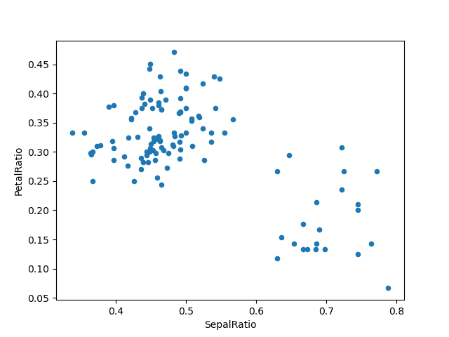
関数が渡されるため、関数は割り当てられるDataFrame上で計算されます。重要なのは、これはsepal lengthが5より大きい行にフィルター処理されたDataFrameです。最初にフィルター処理が行われ、次に比率計算が行われます。これは、フィルター処理されたDataFrameへの参照が利用できなかった例です。
assign()の関数シグネチャは単に**kwargsです。キーは新しいフィールドの列名であり、値は挿入する値(たとえば、SeriesまたはNumPy配列)か、DataFrameに対して呼び出される1引数関数です。新しい値が挿入された、元のDataFrameのコピーが返されます。
**kwargsの順序は保持されます。これにより、**kwargsの後の方の式が、同じassign()で以前に作成された列を参照できるような、依存割り当てが可能になります。
In [90]: dfa = pd.DataFrame({"A": [1, 2, 3], "B": [4, 5, 6]})

In [91]: dfa.assign(C=lambda x: x["A"] + x["B"], D=lambda x: x["A"] + x["C"])
Out[91]:
   A  B  C   D
0  1  4  5   6
1  2  5  7   9
2  3  6  9  12
2番目の式では、x['C']は新しく作成された列を参照し、それはdfa['A'] + dfa['B']と等しくなります。
インデックス付け / 選択#
インデックス付けの基本は以下の通りです。
操作 |
構文 |
結果 |
|---|---|---|
列を選択 |
|
Series |
ラベルで行を選択 |
|
Series |
整数位置で行を選択 |
|
Series |
行をスライス |
|
DataFrame |
ブールベクトルで行を選択 |
|
DataFrame |
たとえば、行選択は、インデックスがDataFrameの列であるSeriesを返します。
In [92]: df.loc["b"]
Out[92]:
one            2.0
bar            2.0
flag         False
foo            bar
one_trunc      2.0
Name: b, dtype: object

In [93]: df.iloc[2]
Out[93]:
one           3.0
bar           3.0
flag         True
foo           bar
one_trunc     NaN
Name: c, dtype: object
洗練されたラベルベースのインデックス付けとスライスに関するより詳細な説明については、インデックス付けのセクションを参照してください。新しいラベルセットへの再インデックス付け / 適応の基本については、再インデックス付けのセクションで説明します。
データアライメントと演算#
DataFrameオブジェクト間のデータアライメントは、列とインデックス(行ラベル)の両方で自動的に行われます。ここでも、結果のオブジェクトは列ラベルと行ラベルのユニオンを持ちます。
In [94]: df = pd.DataFrame(np.random.randn(10, 4), columns=["A", "B", "C", "D"])

In [95]: df2 = pd.DataFrame(np.random.randn(7, 3), columns=["A", "B", "C"])

In [96]: df + df2
Out[96]:
          A         B         C   D
0  0.045691 -0.014138  1.380871 NaN
1 -0.955398 -1.501007  0.037181 NaN
2 -0.662690  1.534833 -0.859691 NaN
3 -2.452949  1.237274 -0.133712 NaN
4  1.414490  1.951676 -2.320422 NaN
5 -0.494922 -1.649727 -1.084601 NaN
6 -1.047551 -0.748572 -0.805479 NaN
7       NaN       NaN       NaN NaN
8       NaN       NaN       NaN NaN
9       NaN       NaN       NaN NaN
DataFrameとSeriesの間で操作を行う場合、デフォルトの動作ではSeriesのインデックスをDataFrameの列に合わせ、行方向にブロードキャストします。例を挙げます。
In [97]: df - df.iloc[0]
Out[97]:
          A         B         C         D
0  0.000000  0.000000  0.000000  0.000000
1 -1.359261 -0.248717 -0.453372 -1.754659
2  0.253128  0.829678  0.010026 -1.991234
3 -1.311128  0.054325 -1.724913 -1.620544
4  0.573025  1.500742 -0.676070  1.367331
5 -1.741248  0.781993 -1.241620 -2.053136
6 -1.240774 -0.869551 -0.153282  0.000430
7 -0.743894  0.411013 -0.929563 -0.282386
8 -1.194921  1.320690  0.238224 -1.482644
9  2.293786  1.856228  0.773289 -1.446531
マッチングとブロードキャストの動作を明示的に制御するには、柔軟な二項演算のセクションを参照してください。
スカラーとの算術演算は要素ごとに機能します。
In [98]: df * 5 + 2
Out[98]:
           A         B         C          D
0   3.359299 -0.124862  4.835102   3.381160
1  -3.437003 -1.368449  2.568242  -5.392133
2   4.624938  4.023526  4.885230  -6.575010
3  -3.196342  0.146766 -3.789461  -4.721559
4   6.224426  7.378849  1.454750  10.217815
5  -5.346940  3.785103 -1.373001  -6.884519
6  -2.844569 -4.472618  4.068691   3.383309
7  -0.360173  1.930201  0.187285   1.969232
8  -2.615303  6.478587  6.026220  -4.032059
9  14.828230  9.156280  8.701544  -3.851494

In [99]: 1 / df
Out[99]:
          A          B         C           D
0  3.678365  -2.353094  1.763605    3.620145
1 -0.919624  -1.484363  8.799067   -0.676395
2  1.904807   2.470934  1.732964   -0.583090
3 -0.962215  -2.697986 -0.863638   -0.743875
4  1.183593   0.929567 -9.170108    0.608434
5 -0.680555   2.800959 -1.482360   -0.562777
6 -1.032084  -0.772485  2.416988    3.614523
7 -2.118489 -71.634509 -2.758294 -162.507295
8 -1.083352   1.116424  1.241860   -0.828904
9  0.389765   0.698687  0.746097   -0.854483

In [100]: df ** 4
Out[100]:
           A             B         C             D
0   0.005462  3.261689e-02  0.103370  5.822320e-03
1   1.398165  2.059869e-01  0.000167  4.777482e+00
2   0.075962  2.682596e-02  0.110877  8.650845e+00
3   1.166571  1.887302e-02  1.797515  3.265879e+00
4   0.509555  1.339298e+00  0.000141  7.297019e+00
5   4.661717  1.624699e-02  0.207103  9.969092e+00
6   0.881334  2.808277e+00  0.029302  5.858632e-03
7   0.049647  3.797614e-08  0.017276  1.433866e-09
8   0.725974  6.437005e-01  0.420446  2.118275e+00
9  43.329821  4.196326e+00  3.227153  1.875802e+00
ブール演算子も要素ごとに機能します。
In [101]: df1 = pd.DataFrame({"a": [1, 0, 1], "b": [0, 1, 1]}, dtype=bool)

In [102]: df2 = pd.DataFrame({"a": [0, 1, 1], "b": [1, 1, 0]}, dtype=bool)

In [103]: df1 & df2
Out[103]:
       a      b
0  False  False
1  False   True
2   True  False

In [104]: df1 | df2
Out[104]:
      a     b
0  True  True
1  True  True
2  True  True

In [105]: df1 ^ df2
Out[105]:
       a      b
0   True   True
1   True  False
2  False   True

In [106]: -df1
Out[106]:
       a      b
0  False   True
1   True  False
2  False  False
転置#
転置するには、ndarrayと同様にT属性またはDataFrame.transpose()にアクセスします。
# only show the first 5 rows
In [107]: df[:5].T
Out[107]:
          0         1         2         3         4
A  0.271860 -1.087401  0.524988 -1.039268  0.844885
B -0.424972 -0.673690  0.404705 -0.370647  1.075770
C  0.567020  0.113648  0.577046 -1.157892 -0.109050
D  0.276232 -1.478427 -1.715002 -1.344312  1.643563
NumPy関数とのDataFrame相互運用性#
ほとんどのNumPy関数は、SeriesおよびDataFrameに対して直接呼び出すことができます。
In [108]: np.exp(df)
Out[108]:
           A         B         C         D
0   1.312403  0.653788  1.763006  1.318154
1   0.337092  0.509824  1.120358  0.227996
2   1.690438  1.498861  1.780770  0.179963
3   0.353713  0.690288  0.314148  0.260719
4   2.327710  2.932249  0.896686  5.173571
5   0.230066  1.429065  0.509360  0.169161
6   0.379495  0.274028  1.512461  1.318720
7   0.623732  0.986137  0.695904  0.993865
8   0.397301  2.449092  2.237242  0.299269
9  13.009059  4.183951  3.820223  0.310274

In [109]: np.asarray(df)
Out[109]:
array([[ 0.2719, -0.425 ,  0.567 ,  0.2762],
       [-1.0874, -0.6737,  0.1136, -1.4784],
       [ 0.525 ,  0.4047,  0.577 , -1.715 ],
       [-1.0393, -0.3706, -1.1579, -1.3443],
       [ 0.8449,  1.0758, -0.109 ,  1.6436],
       [-1.4694,  0.357 , -0.6746, -1.7769],
       [-0.9689, -1.2945,  0.4137,  0.2767],
       [-0.472 , -0.014 , -0.3625, -0.0062],
       [-0.9231,  0.8957,  0.8052, -1.2064],
       [ 2.5656,  1.4313,  1.3403, -1.1703]])
DataFrameは、インデックスのセマンティクスとデータモデルがN次元配列とはかなり異なるため、ndarrayのドロップイン置換として機能するように意図されていません。
Seriesは__array_ufunc__を実装しており、NumPyのユニバーサル関数と連携できます。
ufuncはSeriesの基になる配列に適用されます。
In [110]: ser = pd.Series([1, 2, 3, 4])

In [111]: np.exp(ser)
Out[111]:
0     2.718282
1     7.389056
2    20.085537
3    54.598150
dtype: float64
複数のSeriesがufuncに渡されると、操作を実行する前にそれらはアラインされます。
ライブラリの他の部分と同様に、pandasは複数の入力を持つufuncの一部として、ラベル付き入力を自動的にアラインします。たとえば、異なる順序のラベルを持つ2つのSeriesに対してnumpy.remainder()を使用すると、操作の前にアラインが行われます。
In [112]: ser1 = pd.Series([1, 2, 3], index=["a", "b", "c"])

In [113]: ser2 = pd.Series([1, 3, 5], index=["b", "a", "c"])

In [114]: ser1
Out[114]:
a    1
b    2
c    3
dtype: int64

In [115]: ser2
Out[115]:
b    1
a    3
c    5
dtype: int64

In [116]: np.remainder(ser1, ser2)
Out[116]:
a    1
b    0
c    3
dtype: int64
通常通り、2つのインデックスのユニオンが取られ、重複しない値には欠損値が埋められます。
In [117]: ser3 = pd.Series([2, 4, 6], index=["b", "c", "d"])

In [118]: ser3
Out[118]:
b    2
c    4
d    6
dtype: int64

In [119]: np.remainder(ser1, ser3)
Out[119]:
a    NaN
b    0.0
c    3.0
d    NaN
dtype: float64
二項ufuncがSeriesとIndexに適用される場合、Seriesの実装が優先され、Seriesが返されます。
In [120]: ser = pd.Series([1, 2, 3])

In [121]: idx = pd.Index([4, 5, 6])

In [122]: np.maximum(ser, idx)
Out[122]:
0    4
1    5
2    6
dtype: int64
NumPyのufuncは、ndarray以外の配列(例:arrays.SparseArray(疎行列計算参照))によって裏打ちされたSeriesにも安全に適用できます。可能な場合、ufuncは基となるデータをndarrayに変換せずに適用されます。
コンソール表示#
非常に大きなDataFrameは、コンソールに表示するために切り捨てられます。info()を使用して概要を取得することもできます。(baseballデータセットはplyr Rパッケージからのものです)
In [123]: baseball = pd.read_csv("data/baseball.csv")

In [124]: print(baseball)
       id     player  year  stint team  lg  ...    so  ibb  hbp   sh   sf  gidp
0   88641  womacto01  2006      2  CHN  NL  ...   4.0  0.0  0.0  3.0  0.0   0.0
1   88643  schilcu01  2006      1  BOS  AL  ...   1.0  0.0  0.0  0.0  0.0   0.0
..    ...        ...   ...    ...  ...  ..  ...   ...  ...  ...  ...  ...   ...
98  89533   aloumo01  2007      1  NYN  NL  ...  30.0  5.0  2.0  0.0  3.0  13.0
99  89534  alomasa02  2007      1  NYN  NL  ...   3.0  0.0  0.0  0.0  0.0   0.0

[100 rows x 23 columns]

In [125]: baseball.info()
<class 'pandas.core.frame.DataFrame'>
RangeIndex: 100 entries, 0 to 99
Data columns (total 23 columns):
 #   Column  Non-Null Count  Dtype
---  ------  --------------  -----
 0   id      100 non-null    int64
 1   player  100 non-null    object
 2   year    100 non-null    int64
 3   stint   100 non-null    int64
 4   team    100 non-null    object
 5   lg      100 non-null    object
 6   g       100 non-null    int64
 7   ab      100 non-null    int64
 8   r       100 non-null    int64
 9   h       100 non-null    int64
 10  X2b     100 non-null    int64
 11  X3b     100 non-null    int64
 12  hr      100 non-null    int64
 13  rbi     100 non-null    float64
 14  sb      100 non-null    float64
 15  cs      100 non-null    float64
 16  bb      100 non-null    int64
 17  so      100 non-null    float64
 18  ibb     100 non-null    float64
 19  hbp     100 non-null    float64
 20  sh      100 non-null    float64
 21  sf      100 non-null    float64
 22  gidp    100 non-null    float64
dtypes: float64(9), int64(11), object(3)
memory usage: 18.1+ KB
ただし、DataFrame.to_string()を使用すると、DataFrameの表形式の文字列表現が返されますが、常にコンソールの幅に収まるとは限りません。
In [126]: print(baseball.iloc[-20:, :12].to_string())
       id     player  year  stint team  lg    g   ab   r    h  X2b  X3b
80  89474  finlest01  2007      1  COL  NL   43   94   9   17    3    0
81  89480  embreal01  2007      1  OAK  AL    4    0   0    0    0    0
82  89481  edmonji01  2007      1  SLN  NL  117  365  39   92   15    2
83  89482  easleda01  2007      1  NYN  NL   76  193  24   54    6    0
84  89489  delgaca01  2007      1  NYN  NL  139  538  71  139   30    0
85  89493  cormirh01  2007      1  CIN  NL    6    0   0    0    0    0
86  89494  coninje01  2007      2  NYN  NL   21   41   2    8    2    0
87  89495  coninje01  2007      1  CIN  NL   80  215  23   57   11    1
88  89497  clemero02  2007      1  NYA  AL    2    2   0    1    0    0
89  89498  claytro01  2007      2  BOS  AL    8    6   1    0    0    0
90  89499  claytro01  2007      1  TOR  AL   69  189  23   48   14    0
91  89501  cirilje01  2007      2  ARI  NL   28   40   6    8    4    0
92  89502  cirilje01  2007      1  MIN  AL   50  153  18   40    9    2
93  89521  bondsba01  2007      1  SFN  NL  126  340  75   94   14    0
94  89523  biggicr01  2007      1  HOU  NL  141  517  68  130   31    3
95  89525  benitar01  2007      2  FLO  NL   34    0   0    0    0    0
96  89526  benitar01  2007      1  SFN  NL   19    0   0    0    0    0
97  89530  ausmubr01  2007      1  HOU  NL  117  349  38   82   16    3
98  89533   aloumo01  2007      1  NYN  NL   87  328  51  112   19    1
99  89534  alomasa02  2007      1  NYN  NL    8   22   1    3    1    0
ワイドなDataFrameは、デフォルトでは複数行にわたって表示されます。
In [127]: pd.DataFrame(np.random.randn(3, 12))
Out[127]:
         0         1         2   ...        9         10        11
0 -1.226825  0.769804 -1.281247  ... -1.110336 -0.619976  0.149748
1 -0.732339  0.687738  0.176444  ...  1.462696 -1.743161 -0.826591
2 -0.345352  1.314232  0.690579  ...  0.896171 -0.487602 -0.082240

[3 rows x 12 columns]
display.widthオプションを設定することで、1行に表示する量を変更できます。
In [128]: pd.set_option("display.width", 40)  # default is 80

In [129]: pd.DataFrame(np.random.randn(3, 12))
Out[129]:
         0         1         2   ...        9         10        11
0 -2.182937  0.380396  0.084844  ... -0.023688  2.410179  1.450520
1  0.206053 -0.251905 -2.213588  ... -0.025747 -0.988387  0.094055
2  1.262731  1.289997  0.082423  ... -0.281461  0.030711  0.109121

[3 rows x 12 columns]
display.max_colwidthを設定することで、個々の列の最大幅を調整できます。
In [130]: datafile = {
   .....:     "filename": ["filename_01", "filename_02"],
   .....:     "path": [
   .....:         "media/user_name/storage/folder_01/filename_01",
   .....:         "media/user_name/storage/folder_02/filename_02",
   .....:     ],
   .....: }
   .....:

In [131]: pd.set_option("display.max_colwidth", 30)

In [132]: pd.DataFrame(datafile)
Out[132]:
      filename                           path
0  filename_01  media/user_name/storage/fo...
1  filename_02  media/user_name/storage/fo...

In [133]: pd.set_option("display.max_colwidth", 100)

In [134]: pd.DataFrame(datafile)
Out[134]:
      filename                                           path
0  filename_01  media/user_name/storage/folder_01/filename_01
1  filename_02  media/user_name/storage/folder_02/filename_02
expand_frame_reprオプションを使用してこの機能を無効にすることもできます。これにより、テーブルは1つのブロックとして表示されます。
DataFrameの列属性アクセスとIPython補完#
DataFrameの列ラベルが有効なPython変数名である場合、その列は属性のようにアクセスできます。
In [135]: df = pd.DataFrame({"foo1": np.random.randn(5), "foo2": np.random.randn(5)})

In [136]: df
Out[136]:
       foo1      foo2
0  1.126203  0.781836
1 -0.977349 -1.071357
2  1.474071  0.441153
3 -0.064034  2.353925
4 -1.282782  0.583787

In [137]: df.foo1
Out[137]:
0    1.126203
1   -0.977349
2    1.474071
3   -0.064034
4   -1.282782
Name: foo1, dtype: float64
列はIPythonの補完メカニズムにも接続されており、タブ補完が可能です。
In [5]: df.foo<TAB>  # noqa: E225, E999
df.foo1  df.foo2