クックブック#
ここは、便利で短いパンダスのレシピの例とリンクを集めたリポジトリです。ユーザーがこのドキュメントに追加することを奨励します。
このセクションに興味深いリンクやインラインの例を追加することは、素晴らしい 最初のプルリクエスト となります。
Stack-OverflowとGitHubのリンクを補完するために、可能な限り簡略化され、凝縮され、新規ユーザーに優しいインラインの例が挿入されています。多くのリンクには、インラインの例が提供する以上の拡張情報が含まれています。
pandas (pd) と NumPy (np) だけが省略されてインポートされるモジュールです。残りは、新規ユーザーのために明示的にインポートされたままです。
イディオム#
これらはいくつかの気の利いたpandasのイディオムです。
1つの列に対するif-then/if-then-else、および1つ以上の他の列への代入
In [1]: df = pd.DataFrame(
   ...:     {"AAA": [4, 5, 6, 7], "BBB": [10, 20, 30, 40], "CCC": [100, 50, -30, -50]}
   ...: )
   ...:

In [2]: df
Out[2]:
   AAA  BBB  CCC
0    4   10  100
1    5   20   50
2    6   30  -30
3    7   40  -50
if-then…#
1つの列に対するif-then
In [3]: df.loc[df.AAA >= 5, "BBB"] = -1

In [4]: df
Out[4]:
   AAA  BBB  CCC
0    4   10  100
1    5   -1   50
2    6   -1  -30
3    7   -1  -50
2つの列への代入を伴うif-then
In [5]: df.loc[df.AAA >= 5, ["BBB", "CCC"]] = 555

In [6]: df
Out[6]:
   AAA  BBB  CCC
0    4   10  100
1    5  555  555
2    6  555  555
3    7  555  555
-else を行うために、異なるロジックの別の行を追加します。
In [7]: df.loc[df.AAA < 5, ["BBB", "CCC"]] = 2000

In [8]: df
Out[8]:
   AAA   BBB   CCC
0    4  2000  2000
1    5   555   555
2    6   555   555
3    7   555   555
または、マスクを設定した後で pandas の where を使用します。
In [9]: df_mask = pd.DataFrame(
   ...:     {"AAA": [True] * 4, "BBB": [False] * 4, "CCC": [True, False] * 2}
   ...: )
   ...:

In [10]: df.where(df_mask, -1000)
Out[10]:
   AAA   BBB   CCC
0    4 -1000  2000
1    5 -1000 -1000
2    6 -1000   555
3    7 -1000 -1000
NumPyのwhere()を使用したif-then-else
In [11]: df = pd.DataFrame(
   ....:     {"AAA": [4, 5, 6, 7], "BBB": [10, 20, 30, 40], "CCC": [100, 50, -30, -50]}
   ....: )
   ....:

In [12]: df
Out[12]:
   AAA  BBB  CCC
0    4   10  100
1    5   20   50
2    6   30  -30
3    7   40  -50

In [13]: df["logic"] = np.where(df["AAA"] > 5, "high", "low")

In [14]: df
Out[14]:
   AAA  BBB  CCC logic
0    4   10  100   low
1    5   20   50   low
2    6   30  -30  high
3    7   40  -50  high
分割#
In [15]: df = pd.DataFrame(
   ....:     {"AAA": [4, 5, 6, 7], "BBB": [10, 20, 30, 40], "CCC": [100, 50, -30, -50]}
   ....: )
   ....:

In [16]: df
Out[16]:
   AAA  BBB  CCC
0    4   10  100
1    5   20   50
2    6   30  -30
3    7   40  -50

In [17]: df[df.AAA <= 5]
Out[17]:
   AAA  BBB  CCC
0    4   10  100
1    5   20   50

In [18]: df[df.AAA > 5]
Out[18]:
   AAA  BBB  CCC
2    6   30  -30
3    7   40  -50
基準の構築#
In [19]: df = pd.DataFrame(
   ....:     {"AAA": [4, 5, 6, 7], "BBB": [10, 20, 30, 40], "CCC": [100, 50, -30, -50]}
   ....: )
   ....:

In [20]: df
Out[20]:
   AAA  BBB  CCC
0    4   10  100
1    5   20   50
2    6   30  -30
3    7   40  -50
…および (代入なしで Series を返す)
In [21]: df.loc[(df["BBB"] < 25) & (df["CCC"] >= -40), "AAA"]
Out[21]:
0    4
1    5
Name: AAA, dtype: int64
…または (代入なしで Series を返す)
In [22]: df.loc[(df["BBB"] > 25) | (df["CCC"] >= -40), "AAA"]
Out[22]:
0    4
1    5
2    6
3    7
Name: AAA, dtype: int64
…または (代入ありで DataFrame を変更する)
In [23]: df.loc[(df["BBB"] > 25) | (df["CCC"] >= 75), "AAA"] = 999

In [24]: df
Out[24]:
   AAA  BBB  CCC
0  999   10  100
1    5   20   50
2  999   30  -30
3  999   40  -50
argsortを使用して、特定の値に最も近いデータを含む行を選択します。
In [25]: df = pd.DataFrame(
   ....:     {"AAA": [4, 5, 6, 7], "BBB": [10, 20, 30, 40], "CCC": [100, 50, -30, -50]}
   ....: )
   ....:

In [26]: df
Out[26]:
   AAA  BBB  CCC
0    4   10  100
1    5   20   50
2    6   30  -30
3    7   40  -50

In [27]: aValue = 43.0

In [28]: df.loc[(df.CCC - aValue).abs().argsort()]
Out[28]:
   AAA  BBB  CCC
1    5   20   50
0    4   10  100
2    6   30  -30
3    7   40  -50
In [29]: df = pd.DataFrame(
   ....:     {"AAA": [4, 5, 6, 7], "BBB": [10, 20, 30, 40], "CCC": [100, 50, -30, -50]}
   ....: )
   ....:

In [30]: df
Out[30]:
   AAA  BBB  CCC
0    4   10  100
1    5   20   50
2    6   30  -30
3    7   40  -50

In [31]: Crit1 = df.AAA <= 5.5

In [32]: Crit2 = df.BBB == 10.0

In [33]: Crit3 = df.CCC > -40.0
ハードコードすることもできます
In [34]: AllCrit = Crit1 & Crit2 & Crit3
…または、動的に構築された基準のリストで実行できます。
In [35]: import functools

In [36]: CritList = [Crit1, Crit2, Crit3]

In [37]: AllCrit = functools.reduce(lambda x, y: x & y, CritList)

In [38]: df[AllCrit]
Out[38]:
   AAA  BBB  CCC
0    4   10  100
選択#
データフレーム#
インデックスのドキュメント。
In [39]: df = pd.DataFrame(
   ....:     {"AAA": [4, 5, 6, 7], "BBB": [10, 20, 30, 40], "CCC": [100, 50, -30, -50]}
   ....: )
   ....:

In [40]: df
Out[40]:
   AAA  BBB  CCC
0    4   10  100
1    5   20   50
2    6   30  -30
3    7   40  -50

In [41]: df[(df.AAA <= 6) & (df.index.isin([0, 2, 4]))]
Out[41]:
   AAA  BBB  CCC
0    4   10  100
2    6   30  -30
ラベル指向のスライスにはlocを、位置スライスにはilocを使用する GH 2904
In [42]: df = pd.DataFrame(
   ....:     {"AAA": [4, 5, 6, 7], "BBB": [10, 20, 30, 40], "CCC": [100, 50, -30, -50]},
   ....:     index=["foo", "bar", "boo", "kar"],
   ....: )
   ....:
2つの明示的なスライス方法と、3つ目の一般的なケースがあります。
位置指向 (Pythonスライススタイル: 終了を含まない)
ラベル指向 (非Pythonスライススタイル: 終了を含む)
汎用 (いずれかのスライススタイル: スライスにラベルまたは位置が含まれるかどうかによる)
In [43]: df.loc["bar":"kar"]  # Label
Out[43]:
     AAA  BBB  CCC
bar    5   20   50
boo    6   30  -30
kar    7   40  -50

# Generic
In [44]: df[0:3]
Out[44]:
     AAA  BBB  CCC
foo    4   10  100
bar    5   20   50
boo    6   30  -30

In [45]: df["bar":"kar"]
Out[45]:
     AAA  BBB  CCC
bar    5   20   50
boo    6   30  -30
kar    7   40  -50
インデックスがゼロ以外の開始または単位以外の増分を持つ整数で構成されている場合、曖昧さが発生します。
In [46]: data = {"AAA": [4, 5, 6, 7], "BBB": [10, 20, 30, 40], "CCC": [100, 50, -30, -50]}

In [47]: df2 = pd.DataFrame(data=data, index=[1, 2, 3, 4])  # Note index starts at 1.

In [48]: df2.iloc[1:3]  # Position-oriented
Out[48]:
   AAA  BBB  CCC
2    5   20   50
3    6   30  -30

In [49]: df2.loc[1:3]  # Label-oriented
Out[49]:
   AAA  BBB  CCC
1    4   10  100
2    5   20   50
3    6   30  -30
In [50]: df = pd.DataFrame(
   ....:     {"AAA": [4, 5, 6, 7], "BBB": [10, 20, 30, 40], "CCC": [100, 50, -30, -50]}
   ....: )
   ....:

In [51]: df
Out[51]:
   AAA  BBB  CCC
0    4   10  100
1    5   20   50
2    6   30  -30
3    7   40  -50

In [52]: df[~((df.AAA <= 6) & (df.index.isin([0, 2, 4])))]
Out[52]:
   AAA  BBB  CCC
1    5   20   50
3    7   40  -50
新しい列#
DataFrame.map(以前はapplymapという名前)を使用して、新しい列を効率的かつ動的に作成する
In [53]: df = pd.DataFrame({"AAA": [1, 2, 1, 3], "BBB": [1, 1, 2, 2], "CCC": [2, 1, 3, 1]})

In [54]: df
Out[54]:
   AAA  BBB  CCC
0    1    1    2
1    2    1    1
2    1    2    3
3    3    2    1

In [55]: source_cols = df.columns  # Or some subset would work too

In [56]: new_cols = [str(x) + "_cat" for x in source_cols]

In [57]: categories = {1: "Alpha", 2: "Beta", 3: "Charlie"}

In [58]: df[new_cols] = df[source_cols].map(categories.get)

In [59]: df
Out[59]:
   AAA  BBB  CCC  AAA_cat BBB_cat  CCC_cat
0    1    1    2    Alpha   Alpha     Beta
1    2    1    1     Beta   Alpha    Alpha
2    1    2    3    Alpha    Beta  Charlie
3    3    2    1  Charlie    Beta    Alpha
groupby で min() を使用する際に他の列を保持する
In [60]: df = pd.DataFrame(
   ....:     {"AAA": [1, 1, 1, 2, 2, 2, 3, 3], "BBB": [2, 1, 3, 4, 5, 1, 2, 3]}
   ....: )
   ....:

In [61]: df
Out[61]:
   AAA  BBB
0    1    2
1    1    1
2    1    3
3    2    4
4    2    5
5    2    1
6    3    2
7    3    3
方法1: idxmin()で最小値のインデックスを取得
In [62]: df.loc[df.groupby("AAA")["BBB"].idxmin()]
Out[62]:
   AAA  BBB
1    1    1
5    2    1
6    3    2
方法2: ソートしてからそれぞれの最初の要素を取得する
In [63]: df.sort_values(by="BBB").groupby("AAA", as_index=False).first()
Out[63]:
   AAA  BBB
0    1    1
1    2    1
2    3    2
インデックスを除けば、同じ結果が得られることに注意してください。
マルチインデックス#
マルチインデックスのドキュメント。
In [64]: df = pd.DataFrame(
   ....:     {
   ....:         "row": [0, 1, 2],
   ....:         "One_X": [1.1, 1.1, 1.1],
   ....:         "One_Y": [1.2, 1.2, 1.2],
   ....:         "Two_X": [1.11, 1.11, 1.11],
   ....:         "Two_Y": [1.22, 1.22, 1.22],
   ....:     }
   ....: )
   ....:

In [65]: df
Out[65]:
   row  One_X  One_Y  Two_X  Two_Y
0    0    1.1    1.2   1.11   1.22
1    1    1.1    1.2   1.11   1.22
2    2    1.1    1.2   1.11   1.22

# As Labelled Index
In [66]: df = df.set_index("row")

In [67]: df
Out[67]:
     One_X  One_Y  Two_X  Two_Y
row
0      1.1    1.2   1.11   1.22
1      1.1    1.2   1.11   1.22
2      1.1    1.2   1.11   1.22

# With Hierarchical Columns
In [68]: df.columns = pd.MultiIndex.from_tuples([tuple(c.split("_")) for c in df.columns])

In [69]: df
Out[69]:
     One        Two
       X    Y     X     Y
row
0    1.1  1.2  1.11  1.22
1    1.1  1.2  1.11  1.22
2    1.1  1.2  1.11  1.22

# Now stack & Reset
In [70]: df = df.stack(0, future_stack=True).reset_index(1)

In [71]: df
Out[71]:
    level_1     X     Y
row
0       One  1.10  1.20
0       Two  1.11  1.22
1       One  1.10  1.20
1       Two  1.11  1.22
2       One  1.10  1.20
2       Two  1.11  1.22

# And fix the labels (Notice the label 'level_1' got added automatically)
In [72]: df.columns = ["Sample", "All_X", "All_Y"]

In [73]: df
Out[73]:
    Sample  All_X  All_Y
row
0      One   1.10   1.20
0      Two   1.11   1.22
1      One   1.10   1.20
1      Two   1.11   1.22
2      One   1.10   1.20
2      Two   1.11   1.22
算術演算#
ブロードキャストが必要なMultiIndexでの算術演算の実行
In [74]: cols = pd.MultiIndex.from_tuples(
   ....:     [(x, y) for x in ["A", "B", "C"] for y in ["O", "I"]]
   ....: )
   ....:

In [75]: df = pd.DataFrame(np.random.randn(2, 6), index=["n", "m"], columns=cols)

In [76]: df
Out[76]:
          A                   B                   C
          O         I         O         I         O         I
n  0.469112 -0.282863 -1.509059 -1.135632  1.212112 -0.173215
m  0.119209 -1.044236 -0.861849 -2.104569 -0.494929  1.071804

In [77]: df = df.div(df["C"], level=1)

In [78]: df
Out[78]:
          A                   B              C
          O         I         O         I    O    I
n  0.387021  1.633022 -1.244983  6.556214  1.0  1.0
m -0.240860 -0.974279  1.741358 -1.963577  1.0  1.0
スライシング#
In [79]: coords = [("AA", "one"), ("AA", "six"), ("BB", "one"), ("BB", "two"), ("BB", "six")]

In [80]: index = pd.MultiIndex.from_tuples(coords)

In [81]: df = pd.DataFrame([11, 22, 33, 44, 55], index, ["MyData"])

In [82]: df
Out[82]:
        MyData
AA one      11
   six      22
BB one      33
   two      44
   six      55
1stレベルと1st軸のインデックスのクロスセクションを取る
# Note : level and axis are optional, and default to zero
In [83]: df.xs("BB", level=0, axis=0)
Out[83]:
     MyData
one      33
two      44
six      55
…そして今度は1st軸の2ndレベルです。
In [84]: df.xs("six", level=1, axis=0)
Out[84]:
    MyData
AA      22
BB      55
xs を使った MultiIndex のスライシング、方法 #2
In [85]: import itertools

In [86]: index = list(itertools.product(["Ada", "Quinn", "Violet"], ["Comp", "Math", "Sci"]))

In [87]: headr = list(itertools.product(["Exams", "Labs"], ["I", "II"]))

In [88]: indx = pd.MultiIndex.from_tuples(index, names=["Student", "Course"])

In [89]: cols = pd.MultiIndex.from_tuples(headr)  # Notice these are un-named

In [90]: data = [[70 + x + y + (x * y) % 3 for x in range(4)] for y in range(9)]

In [91]: df = pd.DataFrame(data, indx, cols)

In [92]: df
Out[92]:
               Exams     Labs
                   I  II    I  II
Student Course
Ada     Comp      70  71   72  73
        Math      71  73   75  74
        Sci       72  75   75  75
Quinn   Comp      73  74   75  76
        Math      74  76   78  77
        Sci       75  78   78  78
Violet  Comp      76  77   78  79
        Math      77  79   81  80
        Sci       78  81   81  81

In [93]: All = slice(None)

In [94]: df.loc["Violet"]
Out[94]:
       Exams     Labs
           I  II    I  II
Course
Comp      76  77   78  79
Math      77  79   81  80
Sci       78  81   81  81

In [95]: df.loc[(All, "Math"), All]
Out[95]:
               Exams     Labs
                   I  II    I  II
Student Course
Ada     Math      71  73   75  74
Quinn   Math      74  76   78  77
Violet  Math      77  79   81  80

In [96]: df.loc[(slice("Ada", "Quinn"), "Math"), All]
Out[96]:
               Exams     Labs
                   I  II    I  II
Student Course
Ada     Math      71  73   75  74
Quinn   Math      74  76   78  77

In [97]: df.loc[(All, "Math"), ("Exams")]
Out[97]:
                 I  II
Student Course
Ada     Math    71  73
Quinn   Math    74  76
Violet  Math    77  79

In [98]: df.loc[(All, "Math"), (All, "II")]
Out[98]:
               Exams Labs
                  II   II
Student Course
Ada     Math      73   74
Quinn   Math      76   77
Violet  Math      79   80
ソート#
特定の列または順序付けられた列のリストでソート(MultiIndex付き)
In [99]: df.sort_values(by=("Labs", "II"), ascending=False)
Out[99]:
               Exams     Labs
                   I  II    I  II
Student Course
Violet  Sci       78  81   81  81
        Math      77  79   81  80
        Comp      76  77   78  79
Quinn   Sci       75  78   78  78
        Math      74  76   78  77
        Comp      73  74   75  76
Ada     Sci       72  75   75  75
        Math      71  73   75  74
        Comp      70  71   72  73
部分選択、ソートの必要性 GH 2995
レベル#
欠損データ#
欠損データのドキュメント。
反転した時系列を前方に埋める
In [100]: df = pd.DataFrame(
   .....:     np.random.randn(6, 1),
   .....:     index=pd.date_range("2013-08-01", periods=6, freq="B"),
   .....:     columns=list("A"),
   .....: )
   .....:

In [101]: df.loc[df.index[3], "A"] = np.nan

In [102]: df
Out[102]:
                   A
2013-08-01  0.721555
2013-08-02 -0.706771
2013-08-05 -1.039575
2013-08-06       NaN
2013-08-07 -0.424972
2013-08-08  0.567020

In [103]: df.bfill()
Out[103]:
                   A
2013-08-01  0.721555
2013-08-02 -0.706771
2013-08-05 -1.039575
2013-08-06 -0.424972
2013-08-07 -0.424972
2013-08-08  0.567020
置換#
グループ化#
グループ化のドキュメント。
aggとは異なり、applyの呼び出し可能オブジェクトはサブDataFrameとして渡され、すべての列にアクセスできます。
In [104]: df = pd.DataFrame(
   .....:     {
   .....:         "animal": "cat dog cat fish dog cat cat".split(),
   .....:         "size": list("SSMMMLL"),
   .....:         "weight": [8, 10, 11, 1, 20, 12, 12],
   .....:         "adult": [False] * 5 + [True] * 2,
   .....:     }
   .....: )
   .....:

In [105]: df
Out[105]:
  animal size  weight  adult
0    cat    S       8  False
1    dog    S      10  False
2    cat    M      11  False
3   fish    M       1  False
4    dog    M      20  False
5    cat    L      12   True
6    cat    L      12   True

# List the size of the animals with the highest weight.
In [106]: df.groupby("animal").apply(lambda subf: subf["size"][subf["weight"].idxmax()], include_groups=False)
Out[106]:
animal
cat     L
dog     M
fish    M
dtype: object
In [107]: gb = df.groupby("animal")

In [108]: gb.get_group("cat")
Out[108]:
  animal size  weight  adult
0    cat    S       8  False
2    cat    M      11  False
5    cat    L      12   True
6    cat    L      12   True
In [109]: def GrowUp(x):
   .....:     avg_weight = sum(x[x["size"] == "S"].weight * 1.5)
   .....:     avg_weight += sum(x[x["size"] == "M"].weight * 1.25)
   .....:     avg_weight += sum(x[x["size"] == "L"].weight)
   .....:     avg_weight /= len(x)
   .....:     return pd.Series(["L", avg_weight, True], index=["size", "weight", "adult"])
   .....:

In [110]: expected_df = gb.apply(GrowUp, include_groups=False)

In [111]: expected_df
Out[111]:
       size   weight  adult
animal
cat       L  12.4375   True
dog       L  20.0000   True
fish      L   1.2500   True
In [112]: S = pd.Series([i / 100.0 for i in range(1, 11)])

In [113]: def cum_ret(x, y):
   .....:     return x * (1 + y)
   .....:

In [114]: def red(x):
   .....:     return functools.reduce(cum_ret, x, 1.0)
   .....:

In [115]: S.expanding().apply(red, raw=True)
Out[115]:
0    1.010000
1    1.030200
2    1.061106
3    1.103550
4    1.158728
5    1.228251
6    1.314229
7    1.419367
8    1.547110
9    1.701821
dtype: float64
In [116]: df = pd.DataFrame({"A": [1, 1, 2, 2], "B": [1, -1, 1, 2]})

In [117]: gb = df.groupby("A")

In [118]: def replace(g):
   .....:     mask = g < 0
   .....:     return g.where(~mask, g[~mask].mean())
   .....:

In [119]: gb.transform(replace)
Out[119]:
   B
0  1
1  1
2  1
3  2
In [120]: df = pd.DataFrame(
   .....:     {
   .....:         "code": ["foo", "bar", "baz"] * 2,
   .....:         "data": [0.16, -0.21, 0.33, 0.45, -0.59, 0.62],
   .....:         "flag": [False, True] * 3,
   .....:     }
   .....: )
   .....:

In [121]: code_groups = df.groupby("code")

In [122]: agg_n_sort_order = code_groups[["data"]].transform("sum").sort_values(by="data")

In [123]: sorted_df = df.loc[agg_n_sort_order.index]

In [124]: sorted_df
Out[124]:
  code  data   flag
1  bar -0.21   True
4  bar -0.59  False
0  foo  0.16  False
3  foo  0.45   True
2  baz  0.33  False
5  baz  0.62   True
In [125]: rng = pd.date_range(start="2014-10-07", periods=10, freq="2min")

In [126]: ts = pd.Series(data=list(range(10)), index=rng)

In [127]: def MyCust(x):
   .....:     if len(x) > 2:
   .....:         return x.iloc[1] * 1.234
   .....:     return pd.NaT
   .....:

In [128]: mhc = {"Mean": "mean", "Max": "max", "Custom": MyCust}

In [129]: ts.resample("5min").apply(mhc)
Out[129]:
                     Mean  Max Custom
2014-10-07 00:00:00   1.0    2  1.234
2014-10-07 00:05:00   3.5    4    NaT
2014-10-07 00:10:00   6.0    7  7.404
2014-10-07 00:15:00   8.5    9    NaT

In [130]: ts
Out[130]:
2014-10-07 00:00:00    0
2014-10-07 00:02:00    1
2014-10-07 00:04:00    2
2014-10-07 00:06:00    3
2014-10-07 00:08:00    4
2014-10-07 00:10:00    5
2014-10-07 00:12:00    6
2014-10-07 00:14:00    7
2014-10-07 00:16:00    8
2014-10-07 00:18:00    9
Freq: 2min, dtype: int64
In [131]: df = pd.DataFrame(
   .....:     {"Color": "Red Red Red Blue".split(), "Value": [100, 150, 50, 50]}
   .....: )
   .....:

In [132]: df
Out[132]:
  Color  Value
0   Red    100
1   Red    150
2   Red     50
3  Blue     50

In [133]: df["Counts"] = df.groupby(["Color"]).transform(len)

In [134]: df
Out[134]:
  Color  Value  Counts
0   Red    100       3
1   Red    150       3
2   Red     50       3
3  Blue     50       1
In [135]: df = pd.DataFrame(
   .....:     {"line_race": [10, 10, 8, 10, 10, 8], "beyer": [99, 102, 103, 103, 88, 100]},
   .....:     index=[
   .....:         "Last Gunfighter",
   .....:         "Last Gunfighter",
   .....:         "Last Gunfighter",
   .....:         "Paynter",
   .....:         "Paynter",
   .....:         "Paynter",
   .....:     ],
   .....: )
   .....:

In [136]: df
Out[136]:
                 line_race  beyer
Last Gunfighter         10     99
Last Gunfighter         10    102
Last Gunfighter          8    103
Paynter                 10    103
Paynter                 10     88
Paynter                  8    100

In [137]: df["beyer_shifted"] = df.groupby(level=0)["beyer"].shift(1)

In [138]: df
Out[138]:
                 line_race  beyer  beyer_shifted
Last Gunfighter         10     99            NaN
Last Gunfighter         10    102           99.0
Last Gunfighter          8    103          102.0
Paynter                 10    103            NaN
Paynter                 10     88          103.0
Paynter                  8    100           88.0
In [139]: df = pd.DataFrame(
   .....:     {
   .....:         "host": ["other", "other", "that", "this", "this"],
   .....:         "service": ["mail", "web", "mail", "mail", "web"],
   .....:         "no": [1, 2, 1, 2, 1],
   .....:     }
   .....: ).set_index(["host", "service"])
   .....:

In [140]: mask = df.groupby(level=0).agg("idxmax")

In [141]: df_count = df.loc[mask["no"]].reset_index()

In [142]: df_count
Out[142]:
    host service  no
0  other     web   2
1   that    mail   1
2   this    mail   2
Pythonのitertools.groupbyのようなグループ化
In [143]: df = pd.DataFrame([0, 1, 0, 1, 1, 1, 0, 1, 1], columns=["A"])

In [144]: df["A"].groupby((df["A"] != df["A"].shift()).cumsum()).groups
Out[144]: {1: [0], 2: [1], 3: [2], 4: [3, 4, 5], 5: [6], 6: [7, 8]}

In [145]: df["A"].groupby((df["A"] != df["A"].shift()).cumsum()).cumsum()
Out[145]:
0    0
1    1
2    0
3    1
4    2
5    3
6    0
7    1
8    2
Name: A, dtype: int64
データの拡張#
分割#
行に含まれるロジックに基づいた区切りを使用して、データフレームのリストを作成し、分割します。
In [146]: df = pd.DataFrame(
   .....:     data={
   .....:         "Case": ["A", "A", "A", "B", "A", "A", "B", "A", "A"],
   .....:         "Data": np.random.randn(9),
   .....:     }
   .....: )
   .....:

In [147]: dfs = list(
   .....:     zip(
   .....:         *df.groupby(
   .....:             (1 * (df["Case"] == "B"))
   .....:             .cumsum()
   .....:             .rolling(window=3, min_periods=1)
   .....:             .median()
   .....:         )
   .....:     )
   .....: )[-1]
   .....:

In [148]: dfs[0]
Out[148]:
  Case      Data
0    A  0.276232
1    A -1.087401
2    A -0.673690
3    B  0.113648

In [149]: dfs[1]
Out[149]:
  Case      Data
4    A -1.478427
5    A  0.524988
6    B  0.404705

In [150]: dfs[2]
Out[150]:
  Case      Data
7    A  0.577046
8    A -1.715002
ピボット#
ピボットのドキュメント。
In [151]: df = pd.DataFrame(
   .....:     data={
   .....:         "Province": ["ON", "QC", "BC", "AL", "AL", "MN", "ON"],
   .....:         "City": [
   .....:             "Toronto",
   .....:             "Montreal",
   .....:             "Vancouver",
   .....:             "Calgary",
   .....:             "Edmonton",
   .....:             "Winnipeg",
   .....:             "Windsor",
   .....:         ],
   .....:         "Sales": [13, 6, 16, 8, 4, 3, 1],
   .....:     }
   .....: )
   .....:

In [152]: table = pd.pivot_table(
   .....:     df,
   .....:     values=["Sales"],
   .....:     index=["Province"],
   .....:     columns=["City"],
   .....:     aggfunc="sum",
   .....:     margins=True,
   .....: )
   .....:

In [153]: table.stack("City", future_stack=True)
Out[153]:
                    Sales
Province City
AL       Calgary      8.0
         Edmonton     4.0
         Montreal     NaN
         Toronto      NaN
         Vancouver    NaN
...                   ...
All      Toronto     13.0
         Vancouver   16.0
         Windsor      1.0
         Winnipeg     3.0
         All         51.0

[48 rows x 1 columns]
In [154]: grades = [48, 99, 75, 80, 42, 80, 72, 68, 36, 78]

In [155]: df = pd.DataFrame(
   .....:     {
   .....:         "ID": ["x%d" % r for r in range(10)],
   .....:         "Gender": ["F", "M", "F", "M", "F", "M", "F", "M", "M", "M"],
   .....:         "ExamYear": [
   .....:             "2007",
   .....:             "2007",
   .....:             "2007",
   .....:             "2008",
   .....:             "2008",
   .....:             "2008",
   .....:             "2008",
   .....:             "2009",
   .....:             "2009",
   .....:             "2009",
   .....:         ],
   .....:         "Class": [
   .....:             "algebra",
   .....:             "stats",
   .....:             "bio",
   .....:             "algebra",
   .....:             "algebra",
   .....:             "stats",
   .....:             "stats",
   .....:             "algebra",
   .....:             "bio",
   .....:             "bio",
   .....:         ],
   .....:         "Participated": [
   .....:             "yes",
   .....:             "yes",
   .....:             "yes",
   .....:             "yes",
   .....:             "no",
   .....:             "yes",
   .....:             "yes",
   .....:             "yes",
   .....:             "yes",
   .....:             "yes",
   .....:         ],
   .....:         "Passed": ["yes" if x > 50 else "no" for x in grades],
   .....:         "Employed": [
   .....:             True,
   .....:             True,
   .....:             True,
   .....:             False,
   .....:             False,
   .....:             False,
   .....:             False,
   .....:             True,
   .....:             True,
   .....:             False,
   .....:         ],
   .....:         "Grade": grades,
   .....:     }
   .....: )
   .....:

In [156]: df.groupby("ExamYear").agg(
   .....:     {
   .....:         "Participated": lambda x: x.value_counts()["yes"],
   .....:         "Passed": lambda x: sum(x == "yes"),
   .....:         "Employed": lambda x: sum(x),
   .....:         "Grade": lambda x: sum(x) / len(x),
   .....:     }
   .....: )
   .....:
Out[156]:
          Participated  Passed  Employed      Grade
ExamYear
2007                 3       2         3  74.000000
2008                 3       3         0  68.500000
2009                 3       2         2  60.666667
年と月のクロス集計を作成するには
In [157]: df = pd.DataFrame(
   .....:     {"value": np.random.randn(36)},
   .....:     index=pd.date_range("2011-01-01", freq="ME", periods=36),
   .....: )
   .....:

In [158]: pd.pivot_table(
   .....:     df, index=df.index.month, columns=df.index.year, values="value", aggfunc="sum"
   .....: )
   .....:
Out[158]:
        2011      2012      2013
1  -1.039268 -0.968914  2.565646
2  -0.370647 -1.294524  1.431256
3  -1.157892  0.413738  1.340309
4  -1.344312  0.276662 -1.170299
5   0.844885 -0.472035 -0.226169
6   1.075770 -0.013960  0.410835
7  -0.109050 -0.362543  0.813850
8   1.643563 -0.006154  0.132003
9  -1.469388 -0.923061 -0.827317
10  0.357021  0.895717 -0.076467
11 -0.674600  0.805244 -1.187678
12 -1.776904 -1.206412  1.130127
適用#
ローリング適用で整理 - 埋め込みリストをMultiIndexフレームに変換する
In [159]: df = pd.DataFrame(
   .....:     data={
   .....:         "A": [[2, 4, 8, 16], [100, 200], [10, 20, 30]],
   .....:         "B": [["a", "b", "c"], ["jj", "kk"], ["ccc"]],
   .....:     },
   .....:     index=["I", "II", "III"],
   .....: )
   .....:

In [160]: def SeriesFromSubList(aList):
   .....:     return pd.Series(aList)
   .....:

In [161]: df_orgz = pd.concat(
   .....:     {ind: row.apply(SeriesFromSubList) for ind, row in df.iterrows()}
   .....: )
   .....:

In [162]: df_orgz
Out[162]:
         0     1     2     3
I   A    2     4     8  16.0
    B    a     b     c   NaN
II  A  100   200   NaN   NaN
    B   jj    kk   NaN   NaN
III A   10  20.0  30.0   NaN
    B  ccc   NaN   NaN   NaN
関数がSeriesからスカラーを返す前にSeriesを計算する、複数列に対するローリング適用
In [163]: df = pd.DataFrame(
   .....:     data=np.random.randn(2000, 2) / 10000,
   .....:     index=pd.date_range("2001-01-01", periods=2000),
   .....:     columns=["A", "B"],
   .....: )
   .....:

In [164]: df
Out[164]:
                   A         B
2001-01-01 -0.000144 -0.000141
2001-01-02  0.000161  0.000102
2001-01-03  0.000057  0.000088
2001-01-04 -0.000221  0.000097
2001-01-05 -0.000201 -0.000041
...              ...       ...
2006-06-19  0.000040 -0.000235
2006-06-20 -0.000123 -0.000021
2006-06-21 -0.000113  0.000114
2006-06-22  0.000136  0.000109
2006-06-23  0.000027  0.000030

[2000 rows x 2 columns]

In [165]: def gm(df, const):
   .....:     v = ((((df["A"] + df["B"]) + 1).cumprod()) - 1) * const
   .....:     return v.iloc[-1]
   .....:

In [166]: s = pd.Series(
   .....:     {
   .....:         df.index[i]: gm(df.iloc[i: min(i + 51, len(df) - 1)], 5)
   .....:         for i in range(len(df) - 50)
   .....:     }
   .....: )
   .....:

In [167]: s
Out[167]:
2001-01-01    0.000930
2001-01-02    0.002615
2001-01-03    0.001281
2001-01-04    0.001117
2001-01-05    0.002772
                ...
2006-04-30    0.003296
2006-05-01    0.002629
2006-05-02    0.002081
2006-05-03    0.004247
2006-05-04    0.003928
Length: 1950, dtype: float64
関数がスカラーを返す複数列へのローリング適用 (出来高加重平均価格)
In [168]: rng = pd.date_range(start="2014-01-01", periods=100)

In [169]: df = pd.DataFrame(
   .....:     {
   .....:         "Open": np.random.randn(len(rng)),
   .....:         "Close": np.random.randn(len(rng)),
   .....:         "Volume": np.random.randint(100, 2000, len(rng)),
   .....:     },
   .....:     index=rng,
   .....: )
   .....:

In [170]: df
Out[170]:
                Open     Close  Volume
2014-01-01 -1.611353 -0.492885    1219
2014-01-02 -3.000951  0.445794    1054
2014-01-03 -0.138359 -0.076081    1381
2014-01-04  0.301568  1.198259    1253
2014-01-05  0.276381 -0.669831    1728
...              ...       ...     ...
2014-04-06 -0.040338  0.937843    1188
2014-04-07  0.359661 -0.285908    1864
2014-04-08  0.060978  1.714814     941
2014-04-09  1.759055 -0.455942    1065
2014-04-10  0.138185 -1.147008    1453

[100 rows x 3 columns]

In [171]: def vwap(bars):
   .....:     return (bars.Close * bars.Volume).sum() / bars.Volume.sum()
   .....:

In [172]: window = 5

In [173]: s = pd.concat(
   .....:     [
   .....:         (pd.Series(vwap(df.iloc[i: i + window]), index=[df.index[i + window]]))
   .....:         for i in range(len(df) - window)
   .....:     ]
   .....: )
   .....:

In [174]: s.round(2)
Out[174]:
2014-01-06    0.02
2014-01-07    0.11
2014-01-08    0.10
2014-01-09    0.07
2014-01-10   -0.29
              ...
2014-04-06   -0.63
2014-04-07   -0.02
2014-04-08   -0.03
2014-04-09    0.34
2014-04-10    0.29
Length: 95, dtype: float64
時系列#
週末を除外し、特定の時間のみを含むdatetime範囲を構築する
列に時間、行に日が入った行列を、時系列の形式で連続した行のシーケンスに変換する。 Python pandas DataFrameを再配置する方法は?
DatetimeIndexの各エントリについて、月の最初の日を計算する
In [175]: dates = pd.date_range("2000-01-01", periods=5)

In [176]: dates.to_period(freq="M").to_timestamp()
Out[176]:
DatetimeIndex(['2000-01-01', '2000-01-01', '2000-01-01', '2000-01-01',
               '2000-01-01'],
              dtype='datetime64[ns]', freq=None)
リサンプリング#
リサンプリングのドキュメント。
値の時間グループ化にTimeGrouperの代わりにGrouperを使用する
Grouperへの有効な頻度引数 時系列
TimeGrouperと別のグループ化を使用してサブグループを作成し、カスタム関数を適用する GH 3791
結合#
結合のドキュメント。
重複するインデックスを持つ2つのデータフレームを連結する (Rのrbindを模倣)
In [177]: rng = pd.date_range("2000-01-01", periods=6)

In [178]: df1 = pd.DataFrame(np.random.randn(6, 3), index=rng, columns=["A", "B", "C"])

In [179]: df2 = df1.copy()
DataFrame の構築によっては、ignore_index が必要になる場合があります。
In [180]: df = pd.concat([df1, df2], ignore_index=True)

In [181]: df
Out[181]:
           A         B         C
0  -0.870117 -0.479265 -0.790855
1   0.144817  1.726395 -0.464535
2  -0.821906  1.597605  0.187307
3  -0.128342 -1.511638 -0.289858
4   0.399194 -1.430030 -0.639760
5   1.115116 -2.012600  1.810662
6  -0.870117 -0.479265 -0.790855
7   0.144817  1.726395 -0.464535
8  -0.821906  1.597605  0.187307
9  -0.128342 -1.511638 -0.289858
10  0.399194 -1.430030 -0.639760
11  1.115116 -2.012600  1.810662
DataFrameの自己結合 GH 2996
In [182]: df = pd.DataFrame(
   .....:     data={
   .....:         "Area": ["A"] * 5 + ["C"] * 2,
   .....:         "Bins": [110] * 2 + [160] * 3 + [40] * 2,
   .....:         "Test_0": [0, 1, 0, 1, 2, 0, 1],
   .....:         "Data": np.random.randn(7),
   .....:     }
   .....: )
   .....:

In [183]: df
Out[183]:
  Area  Bins  Test_0      Data
0    A   110       0 -0.433937
1    A   110       1 -0.160552
2    A   160       0  0.744434
3    A   160       1  1.754213
4    A   160       2  0.000850
5    C    40       0  0.342243
6    C    40       1  1.070599

In [184]: df["Test_1"] = df["Test_0"] - 1

In [185]: pd.merge(
   .....:     df,
   .....:     df,
   .....:     left_on=["Bins", "Area", "Test_0"],
   .....:     right_on=["Bins", "Area", "Test_1"],
   .....:     suffixes=("_L", "_R"),
   .....: )
   .....:
Out[185]:
  Area  Bins  Test_0_L    Data_L  Test_1_L  Test_0_R    Data_R  Test_1_R
0    A   110         0 -0.433937        -1         1 -0.160552         0
1    A   160         0  0.744434        -1         1  1.754213         0
2    A   160         1  1.754213         0         2  0.000850         1
3    C    40         0  0.342243        -1         1  1.070599         0
プロット#
プロットのドキュメント。
IPython Jupyterノートブックで複数のグラフをプロットする
Pandas, Vincent, xlsxwriter を使用して Excel ファイルに埋め込みプロットを生成する
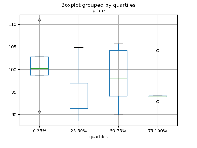
In [186]: df = pd.DataFrame(
   .....:     {
   .....:         "stratifying_var": np.random.uniform(0, 100, 20),
   .....:         "price": np.random.normal(100, 5, 20),
   .....:     }
   .....: )
   .....:

In [187]: df["quartiles"] = pd.qcut(
   .....:     df["stratifying_var"], 4, labels=["0-25%", "25-50%", "50-75%", "75-100%"]
   .....: )
   .....:

In [188]: df.boxplot(column="price", by="quartiles")
Out[188]: <Axes: title={'center': 'price'}, xlabel='quartiles'>
データの入出力#
CSV#
CSVのドキュメント
gzip/bz2 ( read_csv が理解するネイティブな圧縮形式) 以外の方法で圧縮されたファイルを読み込む。この例では WinZipped ファイルを示していますが、コンテキストマネージャー内でファイルを開き、そのハンドルを使用して読み込むという一般的な適用方法です。こちらを参照
不良行の処理 GH 2886
複数のファイルを読み込んで単一のDataFrameを作成する#
複数のファイルを単一のDataFrameに結合する最良の方法は、個々のフレームを1つずつ読み込み、すべての個々のフレームをリストに入れ、次に pd.concat() を使用してリスト内のフレームを結合することです。
In [189]: for i in range(3):
   .....:     data = pd.DataFrame(np.random.randn(10, 4))
   .....:     data.to_csv("file_{}.csv".format(i))
   .....:

In [190]: files = ["file_0.csv", "file_1.csv", "file_2.csv"]

In [191]: result = pd.concat([pd.read_csv(f) for f in files], ignore_index=True)
同じアプローチを使用して、パターンに一致するすべてのファイルを読み取ることができます。ここでは、glob を使用した例を示します。
In [192]: import glob

In [193]: import os

In [194]: files = glob.glob("file_*.csv")

In [195]: result = pd.concat([pd.read_csv(f) for f in files], ignore_index=True)
最後に、この戦略はio docsで説明されている他のpd.read_*(...)関数でも機能します。
複数列での日付コンポーネントの解析#
複数列の日付コンポーネントの解析は、形式を使用すると高速になります。
In [196]: i = pd.date_range("20000101", periods=10000)

In [197]: df = pd.DataFrame({"year": i.year, "month": i.month, "day": i.day})

In [198]: df.head()
Out[198]:
   year  month  day
0  2000      1    1
1  2000      1    2
2  2000      1    3
3  2000      1    4
4  2000      1    5

In [199]: %timeit pd.to_datetime(df.year * 10000 + df.month * 100 + df.day, format='%Y%m%d')
   .....: ds = df.apply(lambda x: "%04d%02d%02d" % (x["year"], x["month"], x["day"]), axis=1)
   .....: ds.head()
   .....: %timeit pd.to_datetime(ds)
   .....:
2.55 ms +- 315 us per loop (mean +- std. dev. of 7 runs, 100 loops each)
1.13 ms +- 10.1 us per loop (mean +- std. dev. of 7 runs, 1,000 loops each)
ヘッダーとデータの間に行をスキップする#
In [200]: data = """;;;;
   .....:  ;;;;
   .....:  ;;;;
   .....:  ;;;;
   .....:  ;;;;
   .....:  ;;;;
   .....: ;;;;
   .....:  ;;;;
   .....:  ;;;;
   .....: ;;;;
   .....: date;Param1;Param2;Param4;Param5
   .....:     ;m²;°C;m²;m
   .....: ;;;;
   .....: 01.01.1990 00:00;1;1;2;3
   .....: 01.01.1990 01:00;5;3;4;5
   .....: 01.01.1990 02:00;9;5;6;7
   .....: 01.01.1990 03:00;13;7;8;9
   .....: 01.01.1990 04:00;17;9;10;11
   .....: 01.01.1990 05:00;21;11;12;13
   .....: """
   .....:
オプション1: スキップする行を明示的に渡す#
In [201]: from io import StringIO

In [202]: pd.read_csv(
   .....:     StringIO(data),
   .....:     sep=";",
   .....:     skiprows=[11, 12],
   .....:     index_col=0,
   .....:     parse_dates=True,
   .....:     header=10,
   .....: )
   .....:
Out[202]:
                     Param1  Param2  Param4  Param5
date
1990-01-01 00:00:00       1       1       2       3
1990-01-01 01:00:00       5       3       4       5
1990-01-01 02:00:00       9       5       6       7
1990-01-01 03:00:00      13       7       8       9
1990-01-01 04:00:00      17       9      10      11
1990-01-01 05:00:00      21      11      12      13
オプション2: 列名を読み込んでからデータを読み込む#
In [203]: pd.read_csv(StringIO(data), sep=";", header=10, nrows=10).columns
Out[203]: Index(['date', 'Param1', 'Param2', 'Param4', 'Param5'], dtype='object')

In [204]: columns = pd.read_csv(StringIO(data), sep=";", header=10, nrows=10).columns

In [205]: pd.read_csv(
   .....:     StringIO(data), sep=";", index_col=0, header=12, parse_dates=True, names=columns
   .....: )
   .....:
Out[205]:
                     Param1  Param2  Param4  Param5
date
1990-01-01 00:00:00       1       1       2       3
1990-01-01 01:00:00       5       3       4       5
1990-01-01 02:00:00       9       5       6       7
1990-01-01 03:00:00      13       7       8       9
1990-01-01 04:00:00      17       9      10      11
1990-01-01 05:00:00      21      11      12      13
SQL#
SQLのドキュメント
Excel#
Excelのドキュメント
表示されているシートのみを読み込む GH 19842#issuecomment-892150745
HTML#
HDFストア#
HDFストアのドキュメント
リンクされた複数テーブル階層を使用して異種データを管理する GH 3032
複数のプロセス/スレッドからストアに書き込む際の不整合を回避する
大規模なストアをチャンクごとに重複排除する、本質的に再帰的な削減操作です。csvファイルからデータを取得し、チャンクごとにストアを作成し、日付解析も行う関数を示しています。こちらを参照
一連のファイルを読み込み、追記しながらストアにグローバルなユニークインデックスを提供する
ptrepackを使用してストア上に完全にソートされたインデックスを作成する
グループノードへの属性の保存
In [206]: df = pd.DataFrame(np.random.randn(8, 3))

In [207]: store = pd.HDFStore("test.h5")

In [208]: store.put("df", df)

# you can store an arbitrary Python object via pickle
In [209]: store.get_storer("df").attrs.my_attribute = {"A": 10}

In [210]: store.get_storer("df").attrs.my_attribute
Out[210]: {'A': 10}
driver パラメータをPyTablesに渡すことで、インメモリでHDFStoreを作成またはロードできます。変更はHDFStoreが閉じられたときにのみディスクに書き込まれます。
In [211]: store = pd.HDFStore("test.h5", "w", driver="H5FD_CORE")

In [212]: df = pd.DataFrame(np.random.randn(8, 3))

In [213]: store["test"] = df

# only after closing the store, data is written to disk:
In [214]: store.close()
バイナリファイル#
C構造体の配列からなるバイナリファイルを読み込む必要がある場合、pandasはNumPyレコード配列を容易に受け入れます。例えば、64ビットマシンでgcc main.c -std=gnu99でコンパイルされたmain.cというファイルにあるこのCプログラムを与えられた場合、
#include <stdio.h>
#include <stdint.h>

typedef struct _Data
{
    int32_t count;
    double avg;
    float scale;
} Data;

int main(int argc, const char *argv[])
{
    size_t n = 10;
    Data d[n];

    for (int i = 0; i < n; ++i)
    {
        d[i].count = i;
        d[i].avg = i + 1.0;
        d[i].scale = (float) i + 2.0f;
    }

    FILE *file = fopen("binary.dat", "wb");
    fwrite(&d, sizeof(Data), n, file);
    fclose(file);

    return 0;
}
以下のPythonコードは、バイナリファイル'binary.dat'をpandasのDataFrameに読み込みます。このDataFrameでは、構造体の各要素がフレームの列に対応します。
names = "count", "avg", "scale"

# note that the offsets are larger than the size of the type because of
# struct padding
offsets = 0, 8, 16
formats = "i4", "f8", "f4"
dt = np.dtype({"names": names, "offsets": offsets, "formats": formats}, align=True)
df = pd.DataFrame(np.fromfile("binary.dat", dt))
注
構造体要素のオフセットは、ファイルが作成されたマシンのアーキテクチャによって異なる場合があります。一般的なデータストレージにこのような生バイナリファイル形式を使用することは、クロスプラットフォームではないため推奨されません。HDF5またはParquetのいずれかを推奨します。どちらもpandasのIO機能によってサポートされています。
計算#
相関#
DataFrame.corr()から計算された相関行列の下(または上)三角形式を取得することがしばしば有用です。これは、次のようにブールマスクをwhereに渡すことで実現できます。
In [215]: df = pd.DataFrame(np.random.random(size=(100, 5)))

In [216]: corr_mat = df.corr()

In [217]: mask = np.tril(np.ones_like(corr_mat, dtype=np.bool_), k=-1)

In [218]: corr_mat.where(mask)
Out[218]:
          0         1         2        3   4
0       NaN       NaN       NaN      NaN NaN
1 -0.079861       NaN       NaN      NaN NaN
2 -0.236573  0.183801       NaN      NaN NaN
3 -0.013795 -0.051975  0.037235      NaN NaN
4 -0.031974  0.118342 -0.073499 -0.02063 NaN
DataFrame.corr内のmethod引数は、指定された相関タイプに加えて呼び出し可能オブジェクトを受け入れることができます。ここでは、DataFrameオブジェクトの距離相関行列を計算します。
In [219]: def distcorr(x, y):
   .....:     n = len(x)
   .....:     a = np.zeros(shape=(n, n))
   .....:     b = np.zeros(shape=(n, n))
   .....:     for i in range(n):
   .....:         for j in range(i + 1, n):
   .....:             a[i, j] = abs(x[i] - x[j])
   .....:             b[i, j] = abs(y[i] - y[j])
   .....:     a += a.T
   .....:     b += b.T
   .....:     a_bar = np.vstack([np.nanmean(a, axis=0)] * n)
   .....:     b_bar = np.vstack([np.nanmean(b, axis=0)] * n)
   .....:     A = a - a_bar - a_bar.T + np.full(shape=(n, n), fill_value=a_bar.mean())
   .....:     B = b - b_bar - b_bar.T + np.full(shape=(n, n), fill_value=b_bar.mean())
   .....:     cov_ab = np.sqrt(np.nansum(A * B)) / n
   .....:     std_a = np.sqrt(np.sqrt(np.nansum(A ** 2)) / n)
   .....:     std_b = np.sqrt(np.sqrt(np.nansum(B ** 2)) / n)
   .....:     return cov_ab / std_a / std_b
   .....:

In [220]: df = pd.DataFrame(np.random.normal(size=(100, 3)))

In [221]: df.corr(method=distcorr)
Out[221]:
          0         1         2
0  1.000000  0.197613  0.216328
1  0.197613  1.000000  0.208749
2  0.216328  0.208749  1.000000
Timedeltas#
Timedeltasのドキュメント。
In [222]: import datetime

In [223]: s = pd.Series(pd.date_range("2012-1-1", periods=3, freq="D"))

In [224]: s - s.max()
Out[224]:
0   -2 days
1   -1 days
2    0 days
dtype: timedelta64[ns]

In [225]: s.max() - s
Out[225]:
0   2 days
1   1 days
2   0 days
dtype: timedelta64[ns]

In [226]: s - datetime.datetime(2011, 1, 1, 3, 5)
Out[226]:
0   364 days 20:55:00
1   365 days 20:55:00
2   366 days 20:55:00
dtype: timedelta64[ns]

In [227]: s + datetime.timedelta(minutes=5)
Out[227]:
0   2012-01-01 00:05:00
1   2012-01-02 00:05:00
2   2012-01-03 00:05:00
dtype: datetime64[ns]

In [228]: datetime.datetime(2011, 1, 1, 3, 5) - s
Out[228]:
0   -365 days +03:05:00
1   -366 days +03:05:00
2   -367 days +03:05:00
dtype: timedelta64[ns]

In [229]: datetime.timedelta(minutes=5) + s
Out[229]:
0   2012-01-01 00:05:00
1   2012-01-02 00:05:00
2   2012-01-03 00:05:00
dtype: datetime64[ns]
In [230]: deltas = pd.Series([datetime.timedelta(days=i) for i in range(3)])

In [231]: df = pd.DataFrame({"A": s, "B": deltas})

In [232]: df
Out[232]:
           A      B
0 2012-01-01 0 days
1 2012-01-02 1 days
2 2012-01-03 2 days

In [233]: df["New Dates"] = df["A"] + df["B"]

In [234]: df["Delta"] = df["A"] - df["New Dates"]

In [235]: df
Out[235]:
           A      B  New Dates   Delta
0 2012-01-01 0 days 2012-01-01  0 days
1 2012-01-02 1 days 2012-01-03 -1 days
2 2012-01-03 2 days 2012-01-05 -2 days

In [236]: df.dtypes
Out[236]:
A             datetime64[ns]
B            timedelta64[ns]
New Dates     datetime64[ns]
Delta        timedelta64[ns]
dtype: object
datetimeと同様に、np.nanを使用して値をNaTに設定できます。
In [237]: y = s - s.shift()

In [238]: y
Out[238]:
0      NaT
1   1 days
2   1 days
dtype: timedelta64[ns]

In [239]: y[1] = np.nan

In [240]: y
Out[240]:
0      NaT
1      NaT
2   1 days
dtype: timedelta64[ns]
例データの作成#
R の expand.grid() 関数のように、いくつかの与えられた値のすべての組み合わせからデータフレームを作成するには、キーが列名で、値がデータ値のリストである辞書を作成できます。
In [241]: def expand_grid(data_dict):
   .....:     rows = itertools.product(*data_dict.values())
   .....:     return pd.DataFrame.from_records(rows, columns=data_dict.keys())
   .....:

In [242]: df = expand_grid(
   .....:     {"height": [60, 70], "weight": [100, 140, 180], "sex": ["Male", "Female"]}
   .....: )
   .....:

In [243]: df
Out[243]:
    height  weight     sex
0       60     100    Male
1       60     100  Female
2       60     140    Male
3       60     140  Female
4       60     180    Male
5       60     180  Female
6       70     100    Male
7       70     100  Female
8       70     140    Male
9       70     140  Female
10      70     180    Male
11      70     180  Female
定数系列#
系列が定数値を持つかどうかを評価するには、series.nunique() <= 1 を確認できます。しかし、最初にすべてのユニークな値をカウントしない、よりパフォーマンスの高いアプローチは次のとおりです。
In [244]: v = s.to_numpy()

In [245]: is_constant = v.shape[0] == 0 or (s[0] == s).all()
このアプローチは、系列に欠損値が含まれていないことを前提としています。NA値を削除する場合、それらの値を最初に削除するだけです。
In [246]: v = s.dropna().to_numpy()

In [247]: is_constant = v.shape[0] == 0 or (s[0] == s).all()
欠損値が他の値と区別されると見なされる場合、次のものを使用できます。
In [248]: v = s.to_numpy()

In [249]: is_constant = v.shape[0] == 0 or (s[0] == s).all() or not pd.notna(v).any()
(この例は、np.nan、pd.NA、およびNoneを区別していないことに注意してください)