データのインデックス付けと選択#
pandasオブジェクト内の軸のラベル情報は、多くの目的に役立ちます。
既知のインジケーターを使用してデータを識別します(つまり、メタデータを提供します)。これは、分析、視覚化、およびインタラクティブなコンソール表示にとって重要です。
自動的および明示的なデータアライメントを可能にします。
データセットのサブセットを直感的に取得および設定できます。
このセクションでは、最後の点に焦点を当てます。つまり、pandasオブジェクトのサブセットをスライス、ダイスし、一般的に取得および設定する方法です。この領域でより多くの開発がなされてきたSeriesとDataFrameが主な焦点となります。
注
PythonとNumPyのインデックス演算子 [] および属性演算子 . は、幅広いユースケースにおいてpandasデータ構造への迅速かつ容易なアクセスを提供します。これにより、Python辞書とNumPy配列の扱い方を知っていれば、新たに学ぶことがほとんどないため、インタラクティブな作業が直感的になります。ただし、アクセスするデータの型が事前にわからないため、標準演算子を直接使用することには最適化の限界があります。プロダクションコードでは、この章で説明する最適化されたpandasデータアクセスメソッドを利用することをお勧めします。
警告
設定操作に対してコピーまたは参照のどちらが返されるかは、コンテキストによって異なる場合があります。これは時として 連鎖割り当て と呼ばれ、避けるべきです。ビューを返すかコピーを返すか を参照してください。
MultiIndex およびより高度なインデックス付けのドキュメントについては、MultiIndex / 高度なインデックス付け を参照してください。
高度な戦略については、クックブック を参照してください。
インデックス付けのさまざまな選択肢#
オブジェクト選択には、より明示的な位置ベースのインデックス付けをサポートするために、ユーザーから多くの追加要望がありました。pandasは現在、3種類の多軸インデックス付けをサポートしています。
.locは主にラベルベースですが、ブール配列と一緒に使用することもできます。.locは、項目が見つからない場合にKeyErrorを発生させます。許容される入力は次のとおりです。単一のラベル。例:
5または'a'(ここで5はインデックスの ラベル として解釈されます。この使用はインデックスに沿った整数位置 ではありません)。ラベルのリストまたは配列
['a', 'b', 'c']。ラベル
'a':'f'を含むスライスオブジェクト (通常のPythonスライスとは異なり、インデックスに存在する場合は開始と停止の 両方 が含まれます! ラベルによるスライス および エンドポイントは包含的 を参照)。ブール配列 (任意の
NA値はFalseとして扱われます)。1つの引数 (呼び出し元のSeriesまたはDataFrame) を取り、インデックス付けに対して有効な出力 (上記のうちの1つ) を返す
callable関数。要素が上記の入力のいずれかである行 (および列) インデックスのタプル。
詳細については、ラベルによる選択 を参照してください。
.ilocは主に整数位置ベース (軸の0からlength-1まで) ですが、ブール配列と一緒に使用することもできます。.ilocは、要求されたインデクサが範囲外の場合にIndexErrorを発生させます。ただし、スライスインデクサは範囲外のインデックス付けを許可します (これはPython/NumPyのスライスセマンティクスに準拠しています)。許容される入力は次のとおりです。整数、例:
5。整数のリストまたは配列
[4, 3, 0]。整数
1:7を含むスライスオブジェクト。ブール配列 (任意の
NA値はFalseとして扱われます)。1つの引数 (呼び出し元のSeriesまたはDataFrame) を取り、インデックス付けに対して有効な出力 (上記のうちの1つ) を返す
callable関数。要素が上記の入力のいずれかである行 (および列) インデックスのタプル。
詳細については、位置による選択、高度なインデックス付け、および 高度な階層 を参照してください。
.loc、.iloc、および[]インデックス付けもインデクサとしてcallableを受け入れることができます。詳細については、Callableによる選択 を参照してください。注
行(および列)インデックスへのタプルキーの分解は、呼び出し可能オブジェクトが適用される 前に 発生するため、行と列の両方をインデックス付けするために呼び出し可能オブジェクトからタプルを返すことはできません。
多軸選択でオブジェクトから値を取得するには、次の表記法を使用します(例として .loc を使用しますが、.iloc にも適用されます)。任意の軸アクセサはヌルスライス : であっても構いません。指定から省略された軸は : と見なされます。例えば、p.loc['a'] は p.loc['a', :] と同等です。
In [1]: ser = pd.Series(range(5), index=list("abcde"))

In [2]: ser.loc[["a", "c", "e"]]
Out[2]:
a    0
c    2
e    4
dtype: int64

In [3]: df = pd.DataFrame(np.arange(25).reshape(5, 5), index=list("abcde"), columns=list("abcde"))

In [4]: df.loc[["a", "c", "e"], ["b", "d"]]
Out[4]:
    b   d
a   1   3
c  11  13
e  21  23
基本#
前のセクション でデータ構造を紹介した際に述べたように、[] (Pythonでクラスの動作を実装することに慣れている人にとっては __getitem__ とも呼ばれる) を用いたインデックス付けの主な機能は、低次元のスライスを選択することです。次の表は、[] を用いてpandasオブジェクトをインデックス付けしたときの戻り値の型を示しています。
オブジェクトの型 |
選択 |
戻り値の型 |
|---|---|---|
Series |
|
スカラ値 |
DataFrame |
|
列名に対応する |
ここでは、インデックス付け機能を説明するために、簡単な時系列データセットを構築します。
In [5]: dates = pd.date_range('1/1/2000', periods=8)

In [6]: df = pd.DataFrame(np.random.randn(8, 4),
   ...:                   index=dates, columns=['A', 'B', 'C', 'D'])
   ...:

In [7]: df
Out[7]:
                   A         B         C         D
2000-01-01  0.469112 -0.282863 -1.509059 -1.135632
2000-01-02  1.212112 -0.173215  0.119209 -1.044236
2000-01-03 -0.861849 -2.104569 -0.494929  1.071804
2000-01-04  0.721555 -0.706771 -1.039575  0.271860
2000-01-05 -0.424972  0.567020  0.276232 -1.087401
2000-01-06 -0.673690  0.113648 -1.478427  0.524988
2000-01-07  0.404705  0.577046 -1.715002 -1.039268
2000-01-08 -0.370647 -1.157892 -1.344312  0.844885
注
特に明記しない限り、インデックス付け機能は時系列に固有のものではありません。
したがって、上記のように、[] を使用した最も基本的なインデックス付けを行います。
In [8]: s = df['A']

In [9]: s[dates[5]]
Out[9]: -0.6736897080883706
[] に列のリストを渡すことで、その順序で列を選択できます。DataFrameに列が含まれていない場合、例外が発生します。複数の列もこの方法で設定できます。
In [10]: df
Out[10]:
                   A         B         C         D
2000-01-01  0.469112 -0.282863 -1.509059 -1.135632
2000-01-02  1.212112 -0.173215  0.119209 -1.044236
2000-01-03 -0.861849 -2.104569 -0.494929  1.071804
2000-01-04  0.721555 -0.706771 -1.039575  0.271860
2000-01-05 -0.424972  0.567020  0.276232 -1.087401
2000-01-06 -0.673690  0.113648 -1.478427  0.524988
2000-01-07  0.404705  0.577046 -1.715002 -1.039268
2000-01-08 -0.370647 -1.157892 -1.344312  0.844885

In [11]: df[['B', 'A']] = df[['A', 'B']]

In [12]: df
Out[12]:
                   A         B         C         D
2000-01-01 -0.282863  0.469112 -1.509059 -1.135632
2000-01-02 -0.173215  1.212112  0.119209 -1.044236
2000-01-03 -2.104569 -0.861849 -0.494929  1.071804
2000-01-04 -0.706771  0.721555 -1.039575  0.271860
2000-01-05  0.567020 -0.424972  0.276232 -1.087401
2000-01-06  0.113648 -0.673690 -1.478427  0.524988
2000-01-07  0.577046  0.404705 -1.715002 -1.039268
2000-01-08 -1.157892 -0.370647 -1.344312  0.844885
これは、列のサブセットに変換を(インプレースで)適用するのに役立つ場合があります。
警告
pandasは、.loc から Series および DataFrame を設定するときに、すべての軸を整列します。
これは、列の配置が値の割り当ての前に行われるため、df を 変更しません。
In [13]: df[['A', 'B']]
Out[13]:
                   A         B
2000-01-01 -0.282863  0.469112
2000-01-02 -0.173215  1.212112
2000-01-03 -2.104569 -0.861849
2000-01-04 -0.706771  0.721555
2000-01-05  0.567020 -0.424972
2000-01-06  0.113648 -0.673690
2000-01-07  0.577046  0.404705
2000-01-08 -1.157892 -0.370647

In [14]: df.loc[:, ['B', 'A']] = df[['A', 'B']]

In [15]: df[['A', 'B']]
Out[15]:
                   A         B
2000-01-01 -0.282863  0.469112
2000-01-02 -0.173215  1.212112
2000-01-03 -2.104569 -0.861849
2000-01-04 -0.706771  0.721555
2000-01-05  0.567020 -0.424972
2000-01-06  0.113648 -0.673690
2000-01-07  0.577046  0.404705
2000-01-08 -1.157892 -0.370647
列の値を交換する正しい方法は、生の値を使用することです。
In [16]: df.loc[:, ['B', 'A']] = df[['A', 'B']].to_numpy()

In [17]: df[['A', 'B']]
Out[17]:
                   A         B
2000-01-01  0.469112 -0.282863
2000-01-02  1.212112 -0.173215
2000-01-03 -0.861849 -2.104569
2000-01-04  0.721555 -0.706771
2000-01-05 -0.424972  0.567020
2000-01-06 -0.673690  0.113648
2000-01-07  0.404705  0.577046
2000-01-08 -0.370647 -1.157892
ただし、.iloc は位置によって操作されるため、.iloc から Series と DataFrame を設定する場合、pandasは軸を整列しません。
これは、値の代入前に列の配置が行われないため、df を変更します。
In [18]: df[['A', 'B']]
Out[18]:
                   A         B
2000-01-01  0.469112 -0.282863
2000-01-02  1.212112 -0.173215
2000-01-03 -0.861849 -2.104569
2000-01-04  0.721555 -0.706771
2000-01-05 -0.424972  0.567020
2000-01-06 -0.673690  0.113648
2000-01-07  0.404705  0.577046
2000-01-08 -0.370647 -1.157892

In [19]: df.iloc[:, [1, 0]] = df[['A', 'B']]

In [20]: df[['A','B']]
Out[20]:
                   A         B
2000-01-01 -0.282863  0.469112
2000-01-02 -0.173215  1.212112
2000-01-03 -2.104569 -0.861849
2000-01-04 -0.706771  0.721555
2000-01-05  0.567020 -0.424972
2000-01-06  0.113648 -0.673690
2000-01-07  0.577046  0.404705
2000-01-08 -1.157892 -0.370647
属性アクセス#
Series のインデックスまたは DataFrame の列に属性として直接アクセスできます。
In [21]: sa = pd.Series([1, 2, 3], index=list('abc'))

In [22]: dfa = df.copy()
In [23]: sa.b
Out[23]: 2

In [24]: dfa.A
Out[24]:
2000-01-01   -0.282863
2000-01-02   -0.173215
2000-01-03   -2.104569
2000-01-04   -0.706771
2000-01-05    0.567020
2000-01-06    0.113648
2000-01-07    0.577046
2000-01-08   -1.157892
Freq: D, Name: A, dtype: float64
In [25]: sa.a = 5

In [26]: sa
Out[26]:
a    5
b    2
c    3
dtype: int64

In [27]: dfa.A = list(range(len(dfa.index)))  # ok if A already exists

In [28]: dfa
Out[28]:
            A         B         C         D
2000-01-01  0  0.469112 -1.509059 -1.135632
2000-01-02  1  1.212112  0.119209 -1.044236
2000-01-03  2 -0.861849 -0.494929  1.071804
2000-01-04  3  0.721555 -1.039575  0.271860
2000-01-05  4 -0.424972  0.276232 -1.087401
2000-01-06  5 -0.673690 -1.478427  0.524988
2000-01-07  6  0.404705 -1.715002 -1.039268
2000-01-08  7 -0.370647 -1.344312  0.844885

In [29]: dfa['A'] = list(range(len(dfa.index)))  # use this form to create a new column

In [30]: dfa
Out[30]:
            A         B         C         D
2000-01-01  0  0.469112 -1.509059 -1.135632
2000-01-02  1  1.212112  0.119209 -1.044236
2000-01-03  2 -0.861849 -0.494929  1.071804
2000-01-04  3  0.721555 -1.039575  0.271860
2000-01-05  4 -0.424972  0.276232 -1.087401
2000-01-06  5 -0.673690 -1.478427  0.524988
2000-01-07  6  0.404705 -1.715002 -1.039268
2000-01-08  7 -0.370647 -1.344312  0.844885
警告
このアクセスは、インデックス要素が有効なPython識別子である場合にのみ使用できます。たとえば、
s.1は許可されません。有効な識別子の説明については、こちら を参照してください。既存のメソッド名と衝突する場合、属性は利用できません。例えば、
s.minは許可されませんが、s['min']は可能です。同様に、以下のリストのいずれかと競合する場合、属性は利用できません:
index、major_axis、minor_axis、items。これらのいずれの場合でも、標準のインデックス付けは機能します。例えば、
s['1']、s['min']、s['index']は対応する要素または列にアクセスします。
IPython環境を使用している場合、タブ補完を使用してこれらのアクセス可能な属性を表示することもできます。
DataFrameの行に dict を割り当てることもできます。
In [31]: x = pd.DataFrame({'x': [1, 2, 3], 'y': [3, 4, 5]})

In [32]: x.iloc[1] = {'x': 9, 'y': 99}

In [33]: x
Out[33]:
   x   y
0  1   3
1  9  99
2  3   5
属性アクセスを使用してSeriesの既存の要素やDataFrameの列を変更できますが、注意が必要です。属性アクセスを使用して新しい列を作成しようとすると、新しい列ではなく新しい属性が作成され、UserWarning が発生します。
In [34]: df_new = pd.DataFrame({'one': [1., 2., 3.]})

In [35]: df_new.two = [4, 5, 6]

In [36]: df_new
Out[36]:
   one
0  1.0
1  2.0
2  3.0
範囲のスライス#
任意の軸に沿って範囲をスライスする最も堅牢で一貫性のある方法は、.iloc メソッドを詳しく説明する 位置による選択 セクションで説明されています。ここでは、[] 演算子を使用したスライスのセマンティクスを説明します。
Seriesでは、構文はndarrayとまったく同じように機能し、値のスライスと対応するラベルを返します。
In [37]: s[:5]
Out[37]:
2000-01-01    0.469112
2000-01-02    1.212112
2000-01-03   -0.861849
2000-01-04    0.721555
2000-01-05   -0.424972
Freq: D, Name: A, dtype: float64

In [38]: s[::2]
Out[38]:
2000-01-01    0.469112
2000-01-03   -0.861849
2000-01-05   -0.424972
2000-01-07    0.404705
Freq: 2D, Name: A, dtype: float64

In [39]: s[::-1]
Out[39]:
2000-01-08   -0.370647
2000-01-07    0.404705
2000-01-06   -0.673690
2000-01-05   -0.424972
2000-01-04    0.721555
2000-01-03   -0.861849
2000-01-02    1.212112
2000-01-01    0.469112
Freq: -1D, Name: A, dtype: float64
設定も機能することに注意してください。
In [40]: s2 = s.copy()

In [41]: s2[:5] = 0

In [42]: s2
Out[42]:
2000-01-01    0.000000
2000-01-02    0.000000
2000-01-03    0.000000
2000-01-04    0.000000
2000-01-05    0.000000
2000-01-06   -0.673690
2000-01-07    0.404705
2000-01-08   -0.370647
Freq: D, Name: A, dtype: float64
DataFrameでは、[] 内のスライスは 行をスライスします。これは非常に一般的な操作であるため、主に利便性のために提供されています。
In [43]: df[:3]
Out[43]:
                   A         B         C         D
2000-01-01 -0.282863  0.469112 -1.509059 -1.135632
2000-01-02 -0.173215  1.212112  0.119209 -1.044236
2000-01-03 -2.104569 -0.861849 -0.494929  1.071804

In [44]: df[::-1]
Out[44]:
                   A         B         C         D
2000-01-08 -1.157892 -0.370647 -1.344312  0.844885
2000-01-07  0.577046  0.404705 -1.715002 -1.039268
2000-01-06  0.113648 -0.673690 -1.478427  0.524988
2000-01-05  0.567020 -0.424972  0.276232 -1.087401
2000-01-04 -0.706771  0.721555 -1.039575  0.271860
2000-01-03 -2.104569 -0.861849 -0.494929  1.071804
2000-01-02 -0.173215  1.212112  0.119209 -1.044236
2000-01-01 -0.282863  0.469112 -1.509059 -1.135632
ラベルによる選択#
警告
設定操作に対してコピーまたは参照のどちらが返されるかは、コンテキストによって異なる場合があります。これは時として chained assignment と呼ばれ、避けるべきです。ビューを返すかコピーを返すか を参照してください。
警告
.locは、インデックス型と互換性のない(または変換できない)スライサーを提示すると厳密に動作します。例えば、DatetimeIndexで整数を使用する場合などです。これらはTypeErrorを発生させます。In [45]: dfl = pd.DataFrame(np.random.randn(5, 4), ....: columns=list('ABCD'), ....: index=pd.date_range('20130101', periods=5)) ....: In [46]: dfl Out[46]: A B C D 2013-01-01 1.075770 -0.109050 1.643563 -1.469388 2013-01-02 0.357021 -0.674600 -1.776904 -0.968914 2013-01-03 -1.294524 0.413738 0.276662 -0.472035 2013-01-04 -0.013960 -0.362543 -0.006154 -0.923061 2013-01-05 0.895717 0.805244 -1.206412 2.565646 In [47]: dfl.loc[2:3] --------------------------------------------------------------------------- TypeError Traceback (most recent call last) Cell In[47], line 1 ----> 1 dfl.loc[2:3] File ~/work/pandas/pandas/pandas/core/indexing.py:1191, in _LocationIndexer.__getitem__(self, key) 1189 maybe_callable = com.apply_if_callable(key, self.obj) 1190 maybe_callable = self._check_deprecated_callable_usage(key, maybe_callable) -> 1191 return self._getitem_axis(maybe_callable, axis=axis) File ~/work/pandas/pandas/pandas/core/indexing.py:1411, in _LocIndexer._getitem_axis(self, key, axis) 1409 if isinstance(key, slice): 1410 self._validate_key(key, axis) -> 1411 return self._get_slice_axis(key, axis=axis) 1412 elif com.is_bool_indexer(key): 1413 return self._getbool_axis(key, axis=axis) File ~/work/pandas/pandas/pandas/core/indexing.py:1443, in _LocIndexer._get_slice_axis(self, slice_obj, axis) 1440 return obj.copy(deep=False) 1442 labels = obj._get_axis(axis) -> 1443 indexer = labels.slice_indexer(slice_obj.start, slice_obj.stop, slice_obj.step) 1445 if isinstance(indexer, slice): 1446 return self.obj._slice(indexer, axis=axis) File ~/work/pandas/pandas/pandas/core/indexes/datetimes.py:682, in DatetimeIndex.slice_indexer(self, start, end, step) 674 # GH#33146 if start and end are combinations of str and None and Index is not 675 # monotonic, we can not use Index.slice_indexer because it does not honor the 676 # actual elements, is only searching for start and end 677 if ( 678 check_str_or_none(start) 679 or check_str_or_none(end) 680 or self.is_monotonic_increasing 681 ): --> 682 return Index.slice_indexer(self, start, end, step) 684 mask = np.array(True) 685 in_index = True File ~/work/pandas/pandas/pandas/core/indexes/base.py:6678, in Index.slice_indexer(self, start, end, step) 6634 def slice_indexer( 6635 self, 6636 start: Hashable | None = None, 6637 end: Hashable | None = None, 6638 step: int | None = None, 6639 ) -> slice: 6640 """ 6641 Compute the slice indexer for input labels and step. 6642 (...) 6676 slice(1, 3, None) 6677 """ -> 6678 start_slice, end_slice = self.slice_locs(start, end, step=step) 6680 # return a slice 6681 if not is_scalar(start_slice): File ~/work/pandas/pandas/pandas/core/indexes/base.py:6904, in Index.slice_locs(self, start, end, step) 6902 start_slice = None 6903 if start is not None: -> 6904 start_slice = self.get_slice_bound(start, "left") 6905 if start_slice is None: 6906 start_slice = 0 File ~/work/pandas/pandas/pandas/core/indexes/base.py:6819, in Index.get_slice_bound(self, label, side) 6815 original_label = label 6817 # For datetime indices label may be a string that has to be converted 6818 # to datetime boundary according to its resolution. -> 6819 label = self._maybe_cast_slice_bound(label, side) 6821 # we need to look up the label 6822 try: File ~/work/pandas/pandas/pandas/core/indexes/datetimes.py:642, in DatetimeIndex._maybe_cast_slice_bound(self, label, side) 637 if isinstance(label, dt.date) and not isinstance(label, dt.datetime): 638 # Pandas supports slicing with dates, treated as datetimes at midnight. 639 # https://github.com/pandas-dev/pandas/issues/31501 640 label = Timestamp(label).to_pydatetime() --> 642 label = super()._maybe_cast_slice_bound(label, side) 643 self._data._assert_tzawareness_compat(label) 644 return Timestamp(label) File ~/work/pandas/pandas/pandas/core/indexes/datetimelike.py:378, in DatetimeIndexOpsMixin._maybe_cast_slice_bound(self, label, side) 376 return lower if side == "left" else upper 377 elif not isinstance(label, self._data._recognized_scalars): --> 378 self._raise_invalid_indexer("slice", label) 380 return label File ~/work/pandas/pandas/pandas/core/indexes/base.py:4308, in Index._raise_invalid_indexer(self, form, key, reraise) 4306 if reraise is not lib.no_default: 4307 raise TypeError(msg) from reraise -> 4308 raise TypeError(msg) TypeError: cannot do slice indexing on DatetimeIndex with these indexers [2] of type int
スライス内の文字列のようなものは、インデックスの型に変換可能であり、自然なスライスにつながる ことがあります。
In [48]: dfl.loc['20130102':'20130104']
Out[48]:
                   A         B         C         D
2013-01-02  0.357021 -0.674600 -1.776904 -0.968914
2013-01-03 -1.294524  0.413738  0.276662 -0.472035
2013-01-04 -0.013960 -0.362543 -0.006154 -0.923061
pandasは、**純粋なラベルベースのインデックス付け**を行うための一連のメソッドを提供します。これは厳密な包含ベースのプロトコルです。要求されたすべてのラベルはインデックス内に存在する必要があり、存在しない場合は KeyError が発生します。スライスの場合、開始境界 **と** 停止境界の 両方 が、インデックス内に存在すれば 含まれます。整数は有効なラベルですが、それらはラベルを指し、**位置を指しません**。
.loc 属性が主要なアクセス方法です。以下の入力が有効です。
単一のラベル。例:
5または'a'(ここで5はインデックスの ラベル として解釈されます。この使用はインデックスに沿った整数位置 ではありません)。ラベルのリストまたは配列
['a', 'b', 'c']。ラベル
'a':'f'を含むスライスオブジェクト (通常のPythonスライスとは異なり、インデックスに存在する場合は開始と停止の 両方 が含まれます! ラベルによるスライス を参照)。ブール配列。
callable、Callableによる選択 を参照。
In [49]: s1 = pd.Series(np.random.randn(6), index=list('abcdef'))

In [50]: s1
Out[50]:
a    1.431256
b    1.340309
c   -1.170299
d   -0.226169
e    0.410835
f    0.813850
dtype: float64

In [51]: s1.loc['c':]
Out[51]:
c   -1.170299
d   -0.226169
e    0.410835
f    0.813850
dtype: float64

In [52]: s1.loc['b']
Out[52]: 1.3403088497993827
設定も機能することに注意してください。
In [53]: s1.loc['c':] = 0

In [54]: s1
Out[54]:
a    1.431256
b    1.340309
c    0.000000
d    0.000000
e    0.000000
f    0.000000
dtype: float64
DataFrameの場合
In [55]: df1 = pd.DataFrame(np.random.randn(6, 4),
   ....:                    index=list('abcdef'),
   ....:                    columns=list('ABCD'))
   ....:

In [56]: df1
Out[56]:
          A         B         C         D
a  0.132003 -0.827317 -0.076467 -1.187678
b  1.130127 -1.436737 -1.413681  1.607920
c  1.024180  0.569605  0.875906 -2.211372
d  0.974466 -2.006747 -0.410001 -0.078638
e  0.545952 -1.219217 -1.226825  0.769804
f -1.281247 -0.727707 -0.121306 -0.097883

In [57]: df1.loc[['a', 'b', 'd'], :]
Out[57]:
          A         B         C         D
a  0.132003 -0.827317 -0.076467 -1.187678
b  1.130127 -1.436737 -1.413681  1.607920
d  0.974466 -2.006747 -0.410001 -0.078638
ラベルスライスによるアクセス
In [58]: df1.loc['d':, 'A':'C']
Out[58]:
          A         B         C
d  0.974466 -2.006747 -0.410001
e  0.545952 -1.219217 -1.226825
f -1.281247 -0.727707 -0.121306
ラベルを使った断面の取得(df.xs('a') と同じ)
In [59]: df1.loc['a']
Out[59]:
A    0.132003
B   -0.827317
C   -0.076467
D   -1.187678
Name: a, dtype: float64
ブール配列で値を取得する
In [60]: df1.loc['a'] > 0
Out[60]:
A     True
B    False
C    False
D    False
Name: a, dtype: bool

In [61]: df1.loc[:, df1.loc['a'] > 0]
Out[61]:
          A
a  0.132003
b  1.130127
c  1.024180
d  0.974466
e  0.545952
f -1.281247
ブール配列中のNA値は False として伝播します。
In [62]: mask = pd.array([True, False, True, False, pd.NA, False], dtype="boolean")

In [63]: mask
Out[63]:
<BooleanArray>
[True, False, True, False, <NA>, False]
Length: 6, dtype: boolean

In [64]: df1[mask]
Out[64]:
          A         B         C         D
a  0.132003 -0.827317 -0.076467 -1.187678
c  1.024180  0.569605  0.875906 -2.211372
値を明示的に取得する
# this is also equivalent to ``df1.at['a','A']``
In [65]: df1.loc['a', 'A']
Out[65]: 0.13200317033032932
ラベルによるスライス#
.loc をスライスと一緒に使用する場合、開始ラベルと終了ラベルの両方がインデックス内に存在すれば、その両方を含む2つの間に 位置する 要素が返されます。
In [66]: s = pd.Series(list('abcde'), index=[0, 3, 2, 5, 4])

In [67]: s.loc[3:5]
Out[67]:
3    b
2    c
5    d
dtype: object
2つのうち少なくとも1つが存在しないが、インデックスがソートされており、開始ラベルと停止ラベルと比較できる場合、2つの間に ランク付けされる ラベルを選択することによって、スライスは期待どおりに機能します。
In [68]: s.sort_index()
Out[68]:
0    a
2    c
3    b
4    e
5    d
dtype: object

In [69]: s.sort_index().loc[1:6]
Out[69]:
2    c
3    b
4    e
5    d
dtype: object
しかし、2つのうち少なくとも1つが存在せず、**かつ**インデックスがソートされていない場合、エラーが発生します(そうしないと計算コストが高く、また混合型インデックスでは曖昧になる可能性があるため)。例えば、上記の例で s.loc[1:6] は KeyError を発生させます。
この動作の根拠については、エンドポイントは包含的 を参照してください。
In [70]: s = pd.Series(list('abcdef'), index=[0, 3, 2, 5, 4, 2])

In [71]: s.loc[3:5]
Out[71]:
3    b
2    c
5    d
dtype: object
また、インデックスに重複するラベルがあり、**かつ**開始ラベルまたは停止ラベルのいずれかが重複している場合、エラーが発生します。例えば、上記の例で s.loc[2:5] は KeyError を発生させます。
重複するラベルに関する詳細については、重複するラベル を参照してください。
位置による選択#
警告
設定操作に対してコピーまたは参照のどちらが返されるかは、コンテキストによって異なる場合があります。これは時として chained assignment と呼ばれ、避けるべきです。ビューを返すかコピーを返すか を参照してください。
pandasは、**純粋に整数ベースのインデックス付け**を行うための一連のメソッドを提供します。そのセマンティクスはPythonおよびNumPyのスライスに密接に従います。これらは 0-based インデックス付けです。スライスの場合、開始境界は 含まれ、上部境界は 除外されます。非整数、たとえ **有効な** ラベルであっても使用しようとすると IndexError が発生します。
.iloc 属性が主要なアクセス方法です。以下の入力が有効です。
整数、例:
5。整数のリストまたは配列
[4, 3, 0]。整数
1:7を含むスライスオブジェクト。ブール配列。
callable、Callableによる選択 を参照。行(および列)インデックスのタプルで、その要素は上記の型のいずれかです。
In [72]: s1 = pd.Series(np.random.randn(5), index=list(range(0, 10, 2)))

In [73]: s1
Out[73]:
0    0.695775
2    0.341734
4    0.959726
6   -1.110336
8   -0.619976
dtype: float64

In [74]: s1.iloc[:3]
Out[74]:
0    0.695775
2    0.341734
4    0.959726
dtype: float64

In [75]: s1.iloc[3]
Out[75]: -1.110336102891167
設定も機能することに注意してください。
In [76]: s1.iloc[:3] = 0

In [77]: s1
Out[77]:
0    0.000000
2    0.000000
4    0.000000
6   -1.110336
8   -0.619976
dtype: float64
DataFrameの場合
In [78]: df1 = pd.DataFrame(np.random.randn(6, 4),
   ....:                    index=list(range(0, 12, 2)),
   ....:                    columns=list(range(0, 8, 2)))
   ....:

In [79]: df1
Out[79]:
           0         2         4         6
0   0.149748 -0.732339  0.687738  0.176444
2   0.403310 -0.154951  0.301624 -2.179861
4  -1.369849 -0.954208  1.462696 -1.743161
6  -0.826591 -0.345352  1.314232  0.690579
8   0.995761  2.396780  0.014871  3.357427
10 -0.317441 -1.236269  0.896171 -0.487602
整数スライスによる選択
In [80]: df1.iloc[:3]
Out[80]:
          0         2         4         6
0  0.149748 -0.732339  0.687738  0.176444
2  0.403310 -0.154951  0.301624 -2.179861
4 -1.369849 -0.954208  1.462696 -1.743161

In [81]: df1.iloc[1:5, 2:4]
Out[81]:
          4         6
2  0.301624 -2.179861
4  1.462696 -1.743161
6  1.314232  0.690579
8  0.014871  3.357427
整数リストによる選択
In [82]: df1.iloc[[1, 3, 5], [1, 3]]
Out[82]:
           2         6
2  -0.154951 -2.179861
6  -0.345352  0.690579
10 -1.236269 -0.487602
In [83]: df1.iloc[1:3, :]
Out[83]:
          0         2         4         6
2  0.403310 -0.154951  0.301624 -2.179861
4 -1.369849 -0.954208  1.462696 -1.743161
In [84]: df1.iloc[:, 1:3]
Out[84]:
           2         4
0  -0.732339  0.687738
2  -0.154951  0.301624
4  -0.954208  1.462696
6  -0.345352  1.314232
8   2.396780  0.014871
10 -1.236269  0.896171
# this is also equivalent to ``df1.iat[1,1]``
In [85]: df1.iloc[1, 1]
Out[85]: -0.1549507744249032
整数位置による断面の取得(df.xs(1) と同等)
In [86]: df1.iloc[1]
Out[86]:
0    0.403310
2   -0.154951
4    0.301624
6   -2.179861
Name: 2, dtype: float64
範囲外のスライスインデックスは、Python/NumPyと同様に適切に処理されます。
# these are allowed in Python/NumPy.
In [87]: x = list('abcdef')

In [88]: x
Out[88]: ['a', 'b', 'c', 'd', 'e', 'f']

In [89]: x[4:10]
Out[89]: ['e', 'f']

In [90]: x[8:10]
Out[90]: []

In [91]: s = pd.Series(x)

In [92]: s
Out[92]:
0    a
1    b
2    c
3    d
4    e
5    f
dtype: object

In [93]: s.iloc[4:10]
Out[93]:
4    e
5    f
dtype: object

In [94]: s.iloc[8:10]
Out[94]: Series([], dtype: object)
境界を超えるスライスを使用すると、空の軸(例えば、空のDataFrameが返される)になる可能性があることに注意してください。
In [95]: dfl = pd.DataFrame(np.random.randn(5, 2), columns=list('AB'))

In [96]: dfl
Out[96]:
          A         B
0 -0.082240 -2.182937
1  0.380396  0.084844
2  0.432390  1.519970
3 -0.493662  0.600178
4  0.274230  0.132885

In [97]: dfl.iloc[:, 2:3]
Out[97]:
Empty DataFrame
Columns: []
Index: [0, 1, 2, 3, 4]

In [98]: dfl.iloc[:, 1:3]
Out[98]:
          B
0 -2.182937
1  0.084844
2  1.519970
3  0.600178
4  0.132885

In [99]: dfl.iloc[4:6]
Out[99]:
         A         B
4  0.27423  0.132885
境界外の単一インデクサは IndexError を発生させます。任意の要素が境界外のインデクサのリストは IndexError を発生させます。
In [100]: dfl.iloc[[4, 5, 6]]
---------------------------------------------------------------------------
IndexError                                Traceback (most recent call last)
File ~/work/pandas/pandas/pandas/core/indexing.py:1714, in _iLocIndexer._get_list_axis(self, key, axis)
   1713 try:
-> 1714     return self.obj._take_with_is_copy(key, axis=axis)
   1715 except IndexError as err:
   1716     # re-raise with different error message, e.g. test_getitem_ndarray_3d

File ~/work/pandas/pandas/pandas/core/generic.py:4172, in NDFrame._take_with_is_copy(self, indices, axis)
   4163 """
   4164 Internal version of the `take` method that sets the `_is_copy`
   4165 attribute to keep track of the parent dataframe (using in indexing
   (...)
   4170 See the docstring of `take` for full explanation of the parameters.
   4171 """
-> 4172 result = self.take(indices=indices, axis=axis)
   4173 # Maybe set copy if we didn't actually change the index.

File ~/work/pandas/pandas/pandas/core/generic.py:4152, in NDFrame.take(self, indices, axis, **kwargs)
   4148     indices = np.arange(
   4149         indices.start, indices.stop, indices.step, dtype=np.intp
   4150     )
-> 4152 new_data = self._mgr.take(
   4153     indices,
   4154     axis=self._get_block_manager_axis(axis),
   4155     verify=True,
   4156 )
   4157 return self._constructor_from_mgr(new_data, axes=new_data.axes).__finalize__(
   4158     self, method="take"
   4159 )

File ~/work/pandas/pandas/pandas/core/internals/managers.py:891, in BaseBlockManager.take(self, indexer, axis, verify)
    890 n = self.shape[axis]
--> 891 indexer = maybe_convert_indices(indexer, n, verify=verify)
    893 new_labels = self.axes[axis].take(indexer)

File ~/work/pandas/pandas/pandas/core/indexers/utils.py:282, in maybe_convert_indices(indices, n, verify)
    281     if mask.any():
--> 282         raise IndexError("indices are out-of-bounds")
    283 return indices

IndexError: indices are out-of-bounds

The above exception was the direct cause of the following exception:

IndexError                                Traceback (most recent call last)
Cell In[100], line 1
----> 1 dfl.iloc[[4, 5, 6]]

File ~/work/pandas/pandas/pandas/core/indexing.py:1191, in _LocationIndexer.__getitem__(self, key)
   1189 maybe_callable = com.apply_if_callable(key, self.obj)
   1190 maybe_callable = self._check_deprecated_callable_usage(key, maybe_callable)
-> 1191 return self._getitem_axis(maybe_callable, axis=axis)

File ~/work/pandas/pandas/pandas/core/indexing.py:1743, in _iLocIndexer._getitem_axis(self, key, axis)
   1741 # a list of integers
   1742 elif is_list_like_indexer(key):
-> 1743     return self._get_list_axis(key, axis=axis)
   1745 # a single integer
   1746 else:
   1747     key = item_from_zerodim(key)

File ~/work/pandas/pandas/pandas/core/indexing.py:1717, in _iLocIndexer._get_list_axis(self, key, axis)
   1714     return self.obj._take_with_is_copy(key, axis=axis)
   1715 except IndexError as err:
   1716     # re-raise with different error message, e.g. test_getitem_ndarray_3d
-> 1717     raise IndexError("positional indexers are out-of-bounds") from err

IndexError: positional indexers are out-of-bounds
In [101]: dfl.iloc[:, 4]
---------------------------------------------------------------------------
IndexError                                Traceback (most recent call last)
Cell In[101], line 1
----> 1 dfl.iloc[:, 4]

File ~/work/pandas/pandas/pandas/core/indexing.py:1184, in _LocationIndexer.__getitem__(self, key)
   1182     if self._is_scalar_access(key):
   1183         return self.obj._get_value(*key, takeable=self._takeable)
-> 1184     return self._getitem_tuple(key)
   1185 else:
   1186     # we by definition only have the 0th axis
   1187     axis = self.axis or 0

File ~/work/pandas/pandas/pandas/core/indexing.py:1690, in _iLocIndexer._getitem_tuple(self, tup)
   1689 def _getitem_tuple(self, tup: tuple):
-> 1690     tup = self._validate_tuple_indexer(tup)
   1691     with suppress(IndexingError):
   1692         return self._getitem_lowerdim(tup)

File ~/work/pandas/pandas/pandas/core/indexing.py:966, in _LocationIndexer._validate_tuple_indexer(self, key)
    964 for i, k in enumerate(key):
    965     try:
--> 966         self._validate_key(k, i)
    967     except ValueError as err:
    968         raise ValueError(
    969             "Location based indexing can only have "
    970             f"[{self._valid_types}] types"
    971         ) from err

File ~/work/pandas/pandas/pandas/core/indexing.py:1592, in _iLocIndexer._validate_key(self, key, axis)
   1590     return
   1591 elif is_integer(key):
-> 1592     self._validate_integer(key, axis)
   1593 elif isinstance(key, tuple):
   1594     # a tuple should already have been caught by this point
   1595     # so don't treat a tuple as a valid indexer
   1596     raise IndexingError("Too many indexers")

File ~/work/pandas/pandas/pandas/core/indexing.py:1685, in _iLocIndexer._validate_integer(self, key, axis)
   1683 len_axis = len(self.obj._get_axis(axis))
   1684 if key >= len_axis or key < -len_axis:
-> 1685     raise IndexError("single positional indexer is out-of-bounds")

IndexError: single positional indexer is out-of-bounds
callableによる選択#
.loc、.iloc、および [] インデックス付けは、インデクサとして callable を受け入れることができます。callable は、1つの引数(呼び出し元のSeriesまたはDataFrame)を取り、インデックス付けに対して有効な出力を返す関数である必要があります。
注
.iloc インデックス付けの場合、行と列のインデックスのタプル分解が呼び出し可能オブジェクトを適用する 前に 発生するため、呼び出し可能オブジェクトからタプルを返すことはサポートされていません。
In [102]: df1 = pd.DataFrame(np.random.randn(6, 4),
   .....:                    index=list('abcdef'),
   .....:                    columns=list('ABCD'))
   .....:

In [103]: df1
Out[103]:
          A         B         C         D
a -0.023688  2.410179  1.450520  0.206053
b -0.251905 -2.213588  1.063327  1.266143
c  0.299368 -0.863838  0.408204 -1.048089
d -0.025747 -0.988387  0.094055  1.262731
e  1.289997  0.082423 -0.055758  0.536580
f -0.489682  0.369374 -0.034571 -2.484478

In [104]: df1.loc[lambda df: df['A'] > 0, :]
Out[104]:
          A         B         C         D
c  0.299368 -0.863838  0.408204 -1.048089
e  1.289997  0.082423 -0.055758  0.536580

In [105]: df1.loc[:, lambda df: ['A', 'B']]
Out[105]:
          A         B
a -0.023688  2.410179
b -0.251905 -2.213588
c  0.299368 -0.863838
d -0.025747 -0.988387
e  1.289997  0.082423
f -0.489682  0.369374

In [106]: df1.iloc[:, lambda df: [0, 1]]
Out[106]:
          A         B
a -0.023688  2.410179
b -0.251905 -2.213588
c  0.299368 -0.863838
d -0.025747 -0.988387
e  1.289997  0.082423
f -0.489682  0.369374

In [107]: df1[lambda df: df.columns[0]]
Out[107]:
a   -0.023688
b   -0.251905
c    0.299368
d   -0.025747
e    1.289997
f   -0.489682
Name: A, dtype: float64
Series で呼び出し可能インデックス付けを使用できます。
In [108]: df1['A'].loc[lambda s: s > 0]
Out[108]:
c    0.299368
e    1.289997
Name: A, dtype: float64
これらのメソッド/インデクサを使用すると、一時変数を使用せずにデータ選択操作を連鎖させることができます。
In [109]: bb = pd.read_csv('data/baseball.csv', index_col='id')

In [110]: (bb.groupby(['year', 'team']).sum(numeric_only=True)
   .....:    .loc[lambda df: df['r'] > 100])
   .....:
Out[110]:
           stint    g    ab    r    h  X2b  ...     so   ibb   hbp    sh    sf  gidp
year team                                   ...
2007 CIN       6  379   745  101  203   35  ...  127.0  14.0   1.0   1.0  15.0  18.0
     DET       5  301  1062  162  283   54  ...  176.0   3.0  10.0   4.0   8.0  28.0
     HOU       4  311   926  109  218   47  ...  212.0   3.0   9.0  16.0   6.0  17.0
     LAN      11  413  1021  153  293   61  ...  141.0   8.0   9.0   3.0   8.0  29.0
     NYN      13  622  1854  240  509  101  ...  310.0  24.0  23.0  18.0  15.0  48.0
     SFN       5  482  1305  198  337   67  ...  188.0  51.0   8.0  16.0   6.0  41.0
     TEX       2  198   729  115  200   40  ...  140.0   4.0   5.0   2.0   8.0  16.0
     TOR       4  459  1408  187  378   96  ...  265.0  16.0  12.0   4.0  16.0  38.0

[8 rows x 18 columns]
位置ベースとラベルベースのインデックス付けの組み合わせ#
「A」列のインデックスから0番目と2番目の要素を取得したい場合は、次のようにします。
In [111]: dfd = pd.DataFrame({'A': [1, 2, 3],
   .....:                     'B': [4, 5, 6]},
   .....:                    index=list('abc'))
   .....:

In [112]: dfd
Out[112]:
   A  B
a  1  4
b  2  5
c  3  6

In [113]: dfd.loc[dfd.index[[0, 2]], 'A']
Out[113]:
a    1
c    3
Name: A, dtype: int64
これは .iloc を使用して表現することもできます。インデクサの場所を明示的に取得し、位置的 インデックス付けを使用して項目を選択します。
In [114]: dfd.iloc[[0, 2], dfd.columns.get_loc('A')]
Out[114]:
a    1
c    3
Name: A, dtype: int64
複数のインデクサを取得するには、.get_indexer を使用します。
In [115]: dfd.iloc[[0, 2], dfd.columns.get_indexer(['A', 'B'])]
Out[115]:
   A  B
a  1  4
c  3  6
再インデックス付け#
見つからない可能性のある要素を選択するための慣用的な方法は、.reindex() を使用することです。再インデックス付け のセクションも参照してください。
In [116]: s = pd.Series([1, 2, 3])

In [117]: s.reindex([1, 2, 3])
Out[117]:
1    2.0
2    3.0
3    NaN
dtype: float64
あるいは、有効な キーのみを選択したい場合は、次の方法が慣用的で効率的です。これは選択のdtypeを保持することを保証します。
In [118]: labels = [1, 2, 3]

In [119]: s.loc[s.index.intersection(labels)]
Out[119]:
1    2
2    3
dtype: int64
インデックスが重複していると、.reindex() でエラーが発生します。
In [120]: s = pd.Series(np.arange(4), index=['a', 'a', 'b', 'c'])

In [121]: labels = ['c', 'd']

In [122]: s.reindex(labels)
---------------------------------------------------------------------------
ValueError                                Traceback (most recent call last)
Cell In[122], line 1
----> 1 s.reindex(labels)

File ~/work/pandas/pandas/pandas/core/series.py:5164, in Series.reindex(self, index, axis, method, copy, level, fill_value, limit, tolerance)
   5147 @doc(
   5148     NDFrame.reindex,  # type: ignore[has-type]
   5149     klass=_shared_doc_kwargs["klass"],
   (...)
   5162     tolerance=None,
   5163 ) -> Series:
-> 5164     return super().reindex(
   5165         index=index,
   5166         method=method,
   5167         copy=copy,
   5168         level=level,
   5169         fill_value=fill_value,
   5170         limit=limit,
   5171         tolerance=tolerance,
   5172     )

File ~/work/pandas/pandas/pandas/core/generic.py:5629, in NDFrame.reindex(self, labels, index, columns, axis, method, copy, level, fill_value, limit, tolerance)
   5626     return self._reindex_multi(axes, copy, fill_value)
   5628 # perform the reindex on the axes
-> 5629 return self._reindex_axes(
   5630     axes, level, limit, tolerance, method, fill_value, copy
   5631 ).__finalize__(self, method="reindex")

File ~/work/pandas/pandas/pandas/core/generic.py:5652, in NDFrame._reindex_axes(self, axes, level, limit, tolerance, method, fill_value, copy)
   5649     continue
   5651 ax = self._get_axis(a)
-> 5652 new_index, indexer = ax.reindex(
   5653     labels, level=level, limit=limit, tolerance=tolerance, method=method
   5654 )
   5656 axis = self._get_axis_number(a)
   5657 obj = obj._reindex_with_indexers(
   5658     {axis: [new_index, indexer]},
   5659     fill_value=fill_value,
   5660     copy=copy,
   5661     allow_dups=False,
   5662 )

File ~/work/pandas/pandas/pandas/core/indexes/base.py:4436, in Index.reindex(self, target, method, level, limit, tolerance)
   4433     raise ValueError("cannot handle a non-unique multi-index!")
   4434 elif not self.is_unique:
   4435     # GH#42568
-> 4436     raise ValueError("cannot reindex on an axis with duplicate labels")
   4437 else:
   4438     indexer, _ = self.get_indexer_non_unique(target)

ValueError: cannot reindex on an axis with duplicate labels
一般的に、目的のラベルと現在の軸を交差させてから、再インデックス付けを行うことができます。
In [123]: s.loc[s.index.intersection(labels)].reindex(labels)
Out[123]:
c    3.0
d    NaN
dtype: float64
しかし、結果のインデックスが重複している場合でも、これはエラーになります。
In [124]: labels = ['a', 'd']

In [125]: s.loc[s.index.intersection(labels)].reindex(labels)
---------------------------------------------------------------------------
ValueError                                Traceback (most recent call last)
Cell In[125], line 1
----> 1 s.loc[s.index.intersection(labels)].reindex(labels)

File ~/work/pandas/pandas/pandas/core/series.py:5164, in Series.reindex(self, index, axis, method, copy, level, fill_value, limit, tolerance)
   5147 @doc(
   5148     NDFrame.reindex,  # type: ignore[has-type]
   5149     klass=_shared_doc_kwargs["klass"],
   (...)
   5162     tolerance=None,
   5163 ) -> Series:
-> 5164     return super().reindex(
   5165         index=index,
   5166         method=method,
   5167         copy=copy,
   5168         level=level,
   5169         fill_value=fill_value,
   5170         limit=limit,
   5171         tolerance=tolerance,
   5172     )

File ~/work/pandas/pandas/pandas/core/generic.py:5629, in NDFrame.reindex(self, labels, index, columns, axis, method, copy, level, fill_value, limit, tolerance)
   5626     return self._reindex_multi(axes, copy, fill_value)
   5628 # perform the reindex on the axes
-> 5629 return self._reindex_axes(
   5630     axes, level, limit, tolerance, method, fill_value, copy
   5631 ).__finalize__(self, method="reindex")

File ~/work/pandas/pandas/pandas/core/generic.py:5652, in NDFrame._reindex_axes(self, axes, level, limit, tolerance, method, fill_value, copy)
   5649     continue
   5651 ax = self._get_axis(a)
-> 5652 new_index, indexer = ax.reindex(
   5653     labels, level=level, limit=limit, tolerance=tolerance, method=method
   5654 )
   5656 axis = self._get_axis_number(a)
   5657 obj = obj._reindex_with_indexers(
   5658     {axis: [new_index, indexer]},
   5659     fill_value=fill_value,
   5660     copy=copy,
   5661     allow_dups=False,
   5662 )

File ~/work/pandas/pandas/pandas/core/indexes/base.py:4436, in Index.reindex(self, target, method, level, limit, tolerance)
   4433     raise ValueError("cannot handle a non-unique multi-index!")
   4434 elif not self.is_unique:
   4435     # GH#42568
-> 4436     raise ValueError("cannot reindex on an axis with duplicate labels")
   4437 else:
   4438     indexer, _ = self.get_indexer_non_unique(target)

ValueError: cannot reindex on an axis with duplicate labels
ランダムサンプルの選択#
sample() メソッドを使用して、SeriesまたはDataFrameから行または列をランダムに選択します。このメソッドはデフォルトで行をサンプリングし、返す行/列の特定の数、または行の割合を受け入れます。
In [126]: s = pd.Series([0, 1, 2, 3, 4, 5])

# When no arguments are passed, returns 1 row.
In [127]: s.sample()
Out[127]:
4    4
dtype: int64

# One may specify either a number of rows:
In [128]: s.sample(n=3)
Out[128]:
0    0
4    4
1    1
dtype: int64

# Or a fraction of the rows:
In [129]: s.sample(frac=0.5)
Out[129]:
5    5
3    3
1    1
dtype: int64
デフォルトでは、sample は各行を最大1回だけ返しますが、replace オプションを使用して置換サンプリングを行うこともできます。
In [130]: s = pd.Series([0, 1, 2, 3, 4, 5])

# Without replacement (default):
In [131]: s.sample(n=6, replace=False)
Out[131]:
0    0
1    1
5    5
3    3
2    2
4    4
dtype: int64

# With replacement:
In [132]: s.sample(n=6, replace=True)
Out[132]:
0    0
4    4
3    3
2    2
4    4
4    4
dtype: int64
デフォルトでは、各行が選択される確率は同じですが、行に異なる確率を持たせたい場合は、weights としてサンプリングウェイトを sample 関数に渡すことができます。これらのウェイトはリスト、NumPy配列、またはSeriesにすることができますが、サンプリングするオブジェクトと同じ長さである必要があります。欠損値はウェイトゼロとして扱われ、無限大の値は許可されません。ウェイトの合計が1にならない場合、すべてのウェイトをウェイトの合計で割ることによって再正規化されます。例えば
In [133]: s = pd.Series([0, 1, 2, 3, 4, 5])

In [134]: example_weights = [0, 0, 0.2, 0.2, 0.2, 0.4]

In [135]: s.sample(n=3, weights=example_weights)
Out[135]:
5    5
4    4
3    3
dtype: int64

# Weights will be re-normalized automatically
In [136]: example_weights2 = [0.5, 0, 0, 0, 0, 0]

In [137]: s.sample(n=1, weights=example_weights2)
Out[137]:
0    0
dtype: int64
DataFrameに適用する場合、DataFrameの列をサンプリングウェイトとして使用できます(行をサンプリングしていて列をサンプリングしていない場合)—単に列の名前を文字列として渡すだけです。
In [138]: df2 = pd.DataFrame({'col1': [9, 8, 7, 6],
   .....:                     'weight_column': [0.5, 0.4, 0.1, 0]})
   .....:

In [139]: df2.sample(n=3, weights='weight_column')
Out[139]:
   col1  weight_column
1     8            0.4
0     9            0.5
2     7            0.1
sample はまた、axis 引数を使用して行ではなく列をサンプリングすることもできます。
In [140]: df3 = pd.DataFrame({'col1': [1, 2, 3], 'col2': [2, 3, 4]})

In [141]: df3.sample(n=1, axis=1)
Out[141]:
   col1
0     1
1     2
2     3
最後に、sample の乱数ジェネレーターのシードを random_state 引数で設定することもできます。これは整数(シードとして)またはNumPy RandomStateオブジェクトを受け入れます。
In [142]: df4 = pd.DataFrame({'col1': [1, 2, 3], 'col2': [2, 3, 4]})

# With a given seed, the sample will always draw the same rows.
In [143]: df4.sample(n=2, random_state=2)
Out[143]:
   col1  col2
2     3     4
1     2     3

In [144]: df4.sample(n=2, random_state=2)
Out[144]:
   col1  col2
2     3     4
1     2     3
拡大を伴う設定#
.loc/[] 操作は、その軸に存在しないキーを設定するときに拡大を実行できます。
Series の場合、これは実質的に追加操作となります。
In [145]: se = pd.Series([1, 2, 3])

In [146]: se
Out[146]:
0    1
1    2
2    3
dtype: int64

In [147]: se[5] = 5.

In [148]: se
Out[148]:
0    1.0
1    2.0
2    3.0
5    5.0
dtype: float64
DataFrame は .loc を介してどちらの軸でも拡大できます。
In [149]: dfi = pd.DataFrame(np.arange(6).reshape(3, 2),
   .....:                    columns=['A', 'B'])
   .....:

In [150]: dfi
Out[150]:
   A  B
0  0  1
1  2  3
2  4  5

In [151]: dfi.loc[:, 'C'] = dfi.loc[:, 'A']

In [152]: dfi
Out[152]:
   A  B  C
0  0  1  0
1  2  3  2
2  4  5  4
これは DataFrame の append 操作のようなものです。
In [153]: dfi.loc[3] = 5

In [154]: dfi
Out[154]:
   A  B  C
0  0  1  0
1  2  3  2
2  4  5  4
3  5  5  5
高速なスカラー値の取得と設定#
[] によるインデックス付けは、多くのケース(単一ラベルアクセス、スライシング、ブールインデックス付けなど)を処理する必要があるため、何を要求しているかを把握するのに少しオーバーヘッドがあります。スカラー値にのみアクセスしたい場合、最も速い方法は、すべてのデータ構造に実装されている at および iat メソッドを使用することです。
loc と同様に、at は ラベル ベースのスカラー検索を提供し、iat は iloc と同様に 整数 ベースの検索を提供します。
In [155]: s.iat[5]
Out[155]: 5

In [156]: df.at[dates[5], 'A']
Out[156]: 0.1136484096888855

In [157]: df.iat[3, 0]
Out[157]: -0.7067711336300845
これらの同じインデクサを使用して設定することもできます。
In [158]: df.at[dates[5], 'E'] = 7

In [159]: df.iat[3, 0] = 7
インデクサが欠落している場合、at は上記のようにオブジェクトをインプレースで拡大する可能性があります。
In [160]: df.at[dates[-1] + pd.Timedelta('1 day'), 0] = 7

In [161]: df
Out[161]:
                   A         B         C         D    E    0
2000-01-01 -0.282863  0.469112 -1.509059 -1.135632  NaN  NaN
2000-01-02 -0.173215  1.212112  0.119209 -1.044236  NaN  NaN
2000-01-03 -2.104569 -0.861849 -0.494929  1.071804  NaN  NaN
2000-01-04  7.000000  0.721555 -1.039575  0.271860  NaN  NaN
2000-01-05  0.567020 -0.424972  0.276232 -1.087401  NaN  NaN
2000-01-06  0.113648 -0.673690 -1.478427  0.524988  7.0  NaN
2000-01-07  0.577046  0.404705 -1.715002 -1.039268  NaN  NaN
2000-01-08 -1.157892 -0.370647 -1.344312  0.844885  NaN  NaN
2000-01-09       NaN       NaN       NaN       NaN  NaN  7.0
ブールインデックス付け#
もう一つの一般的な操作は、ブールベクトルを使用してデータをフィルタリングすることです。演算子は、or の場合は |、and の場合は &、not の場合は ~ です。これらは、括弧を使用してグループ化 する必要があります。なぜなら、デフォルトではPythonは df['A'] > 2 & df['B'] < 3 のような式を df['A'] > (2 & df['B']) < 3 として評価し、目的の評価順序は (df['A'] > 2) & (df['B'] < 3) だからです。
ブールベクトルでSeriesをインデックス付けすると、NumPy ndarrayとまったく同じように機能します。
In [162]: s = pd.Series(range(-3, 4))

In [163]: s
Out[163]:
0   -3
1   -2
2   -1
3    0
4    1
5    2
6    3
dtype: int64

In [164]: s[s > 0]
Out[164]:
4    1
5    2
6    3
dtype: int64

In [165]: s[(s < -1) | (s > 0.5)]
Out[165]:
0   -3
1   -2
4    1
5    2
6    3
dtype: int64

In [166]: s[~(s < 0)]
Out[166]:
3    0
4    1
5    2
6    3
dtype: int64
DataFrameのインデックスと同じ長さのブールベクトル(例えば、DataFrameの列の1つから派生したもの)を使用してDataFrameから行を選択できます。
In [167]: df[df['A'] > 0]
Out[167]:
                   A         B         C         D    E   0
2000-01-04  7.000000  0.721555 -1.039575  0.271860  NaN NaN
2000-01-05  0.567020 -0.424972  0.276232 -1.087401  NaN NaN
2000-01-06  0.113648 -0.673690 -1.478427  0.524988  7.0 NaN
2000-01-07  0.577046  0.404705 -1.715002 -1.039268  NaN NaN
リスト内包表記とSeriesの map メソッドを使用して、より複雑な条件を作成することもできます。
In [168]: df2 = pd.DataFrame({'a': ['one', 'one', 'two', 'three', 'two', 'one', 'six'],
   .....:                     'b': ['x', 'y', 'y', 'x', 'y', 'x', 'x'],
   .....:                     'c': np.random.randn(7)})
   .....:

# only want 'two' or 'three'
In [169]: criterion = df2['a'].map(lambda x: x.startswith('t'))

In [170]: df2[criterion]
Out[170]:
       a  b         c
2    two  y  0.041290
3  three  x  0.361719
4    two  y -0.238075

# equivalent but slower
In [171]: df2[[x.startswith('t') for x in df2['a']]]
Out[171]:
       a  b         c
2    two  y  0.041290
3  three  x  0.361719
4    two  y -0.238075

# Multiple criteria
In [172]: df2[criterion & (df2['b'] == 'x')]
Out[172]:
       a  b         c
3  three  x  0.361719
ラベルによる選択、位置による選択、および 高度なインデックス付け の選択メソッドを使用すると、ブールベクトルと他のインデックス式を組み合わせて複数の軸に沿って選択できます。
In [173]: df2.loc[criterion & (df2['b'] == 'x'), 'b':'c']
Out[173]:
   b         c
3  x  0.361719
警告
iloc は2種類のブールインデックス付けをサポートしています。インデクサがブール Series の場合、エラーが発生します。例えば、次の例では df.iloc[s.values, 1] は問題ありません。ブールインデクサは配列です。しかし df.iloc[s, 1] は ValueError を発生させます。
In [174]: df = pd.DataFrame([[1, 2], [3, 4], [5, 6]],
   .....:                   index=list('abc'),
   .....:                   columns=['A', 'B'])
   .....:

In [175]: s = (df['A'] > 2)

In [176]: s
Out[176]:
a    False
b     True
c     True
Name: A, dtype: bool

In [177]: df.loc[s, 'B']
Out[177]:
b    4
c    6
Name: B, dtype: int64

In [178]: df.iloc[s.values, 1]
Out[178]:
b    4
c    6
Name: B, dtype: int64
isinによるインデックス付け#
Series の isin() メソッドについて考えてみましょう。これは、Series要素が渡されたリストに存在する場所で真となるブールベクトルを返します。これにより、1つ以上の列に目的の値を持つ行を選択できます。
In [179]: s = pd.Series(np.arange(5), index=np.arange(5)[::-1], dtype='int64')

In [180]: s
Out[180]:
4    0
3    1
2    2
1    3
0    4
dtype: int64

In [181]: s.isin([2, 4, 6])
Out[181]:
4    False
3    False
2     True
1    False
0     True
dtype: bool

In [182]: s[s.isin([2, 4, 6])]
Out[182]:
2    2
0    4
dtype: int64
同じメソッドが Index オブジェクトでも利用でき、探しているラベルのどれが実際に存在するか分からない場合に役立ちます。
In [183]: s[s.index.isin([2, 4, 6])]
Out[183]:
4    0
2    2
dtype: int64

# compare it to the following
In [184]: s.reindex([2, 4, 6])
Out[184]:
2    2.0
4    0.0
6    NaN
dtype: float64
それに加えて、MultiIndex は、メンバーシップチェックに使用する別のレベルを選択することを可能にします。
In [185]: s_mi = pd.Series(np.arange(6),
   .....:                  index=pd.MultiIndex.from_product([[0, 1], ['a', 'b', 'c']]))
   .....:

In [186]: s_mi
Out[186]:
0  a    0
   b    1
   c    2
1  a    3
   b    4
   c    5
dtype: int64

In [187]: s_mi.iloc[s_mi.index.isin([(1, 'a'), (2, 'b'), (0, 'c')])]
Out[187]:
0  c    2
1  a    3
dtype: int64

In [188]: s_mi.iloc[s_mi.index.isin(['a', 'c', 'e'], level=1)]
Out[188]:
0  a    0
   c    2
1  a    3
   c    5
dtype: int64
DataFrameも isin() メソッドを持っています。isin を呼び出す際には、値のセットを配列またはdictとして渡します。値が配列の場合、isin は元のDataFrameと同じ形状のブールDataFrameを返し、要素が値のシーケンスにある場合はTrueとなります。
In [189]: df = pd.DataFrame({'vals': [1, 2, 3, 4], 'ids': ['a', 'b', 'f', 'n'],
   .....:                    'ids2': ['a', 'n', 'c', 'n']})
   .....:

In [190]: values = ['a', 'b', 1, 3]

In [191]: df.isin(values)
Out[191]:
    vals    ids   ids2
0   True   True   True
1  False   True  False
2   True  False  False
3  False  False  False
多くの場合、特定の列に特定の値を対応させたいと思うでしょう。値を、キーが列で、値がチェックしたい項目のリストである dict にするだけです。
In [192]: values = {'ids': ['a', 'b'], 'vals': [1, 3]}

In [193]: df.isin(values)
Out[193]:
    vals    ids   ids2
0   True   True  False
1  False   True  False
2   True  False  False
3  False  False  False
値が元のDataFrameに ない ブール値のDataFrameを返すには、~ 演算子を使用します。
In [194]: values = {'ids': ['a', 'b'], 'vals': [1, 3]}

In [195]: ~df.isin(values)
Out[195]:
    vals    ids  ids2
0  False  False  True
1   True  False  True
2  False   True  True
3   True   True  True
DataFrameの isin を any() および all() メソッドと組み合わせて、与えられた基準を満たすデータのサブセットを迅速に選択します。各列が独自の基準を満たす行を選択するには、次のようにします。
In [196]: values = {'ids': ['a', 'b'], 'ids2': ['a', 'c'], 'vals': [1, 3]}

In [197]: row_mask = df.isin(values).all(1)

In [198]: df[row_mask]
Out[198]:
   vals ids ids2
0     1   a    a
where() メソッドとマスキング#
ブールベクトルでSeriesから値を選択すると、一般的にデータのサブセットが返されます。選択の出力が元のデータと同じ形状であることを保証するには、Series と DataFrame の where メソッドを使用できます。
選択した行のみを返すには
In [199]: s[s > 0]
Out[199]:
3    1
2    2
1    3
0    4
dtype: int64
元のSeriesと同じ形状のSeriesを返すには
In [200]: s.where(s > 0)
Out[200]:
4    NaN
3    1.0
2    2.0
1    3.0
0    4.0
dtype: float64
ブール条件でDataFrameから値を選択する場合も、入力データの形状が維持されます。where は実装として内部で使用されます。以下のコードは df.where(df < 0) と同等です。
In [201]: dates = pd.date_range('1/1/2000', periods=8)

In [202]: df = pd.DataFrame(np.random.randn(8, 4),
   .....:                   index=dates, columns=['A', 'B', 'C', 'D'])
   .....:

In [203]: df[df < 0]
Out[203]:
                   A         B         C         D
2000-01-01 -2.104139 -1.309525       NaN       NaN
2000-01-02 -0.352480       NaN -1.192319       NaN
2000-01-03 -0.864883       NaN -0.227870       NaN
2000-01-04       NaN -1.222082       NaN -1.233203
2000-01-05       NaN -0.605656 -1.169184       NaN
2000-01-06       NaN -0.948458       NaN -0.684718
2000-01-07 -2.670153 -0.114722       NaN -0.048048
2000-01-08       NaN       NaN -0.048788 -0.808838
さらに、where はオプションの other 引数を受け入れ、返されるコピーで条件がFalseの場合の値を置き換えます。
In [204]: df.where(df < 0, -df)
Out[204]:
                   A         B         C         D
2000-01-01 -2.104139 -1.309525 -0.485855 -0.245166
2000-01-02 -0.352480 -0.390389 -1.192319 -1.655824
2000-01-03 -0.864883 -0.299674 -0.227870 -0.281059
2000-01-04 -0.846958 -1.222082 -0.600705 -1.233203
2000-01-05 -0.669692 -0.605656 -1.169184 -0.342416
2000-01-06 -0.868584 -0.948458 -2.297780 -0.684718
2000-01-07 -2.670153 -0.114722 -0.168904 -0.048048
2000-01-08 -0.801196 -1.392071 -0.048788 -0.808838
いくつかのブール条件に基づいて値を設定したい場合があります。これは次のように直感的に行うことができます。
In [205]: s2 = s.copy()

In [206]: s2[s2 < 0] = 0

In [207]: s2
Out[207]:
4    0
3    1
2    2
1    3
0    4
dtype: int64

In [208]: df2 = df.copy()

In [209]: df2[df2 < 0] = 0

In [210]: df2
Out[210]:
                   A         B         C         D
2000-01-01  0.000000  0.000000  0.485855  0.245166
2000-01-02  0.000000  0.390389  0.000000  1.655824
2000-01-03  0.000000  0.299674  0.000000  0.281059
2000-01-04  0.846958  0.000000  0.600705  0.000000
2000-01-05  0.669692  0.000000  0.000000  0.342416
2000-01-06  0.868584  0.000000  2.297780  0.000000
2000-01-07  0.000000  0.000000  0.168904  0.000000
2000-01-08  0.801196  1.392071  0.000000  0.000000
where は、データの変更されたコピーを返します。
注
DataFrame.where() のシグネチャは numpy.where() と異なります。おおよそ df1.where(m, df2) は np.where(m, df1, df2) と同等です。
In [211]: df.where(df < 0, -df) == np.where(df < 0, df, -df)
Out[211]:
               A     B     C     D
2000-01-01  True  True  True  True
2000-01-02  True  True  True  True
2000-01-03  True  True  True  True
2000-01-04  True  True  True  True
2000-01-05  True  True  True  True
2000-01-06  True  True  True  True
2000-01-07  True  True  True  True
2000-01-08  True  True  True  True
アライメント
さらに、where は入力ブール条件 (ndarray または DataFrame) を整列するため、設定を伴う部分選択が可能です。これは、.loc を介した部分設定 (軸ラベルではなく内容に対して) と同様です。
In [212]: df2 = df.copy()

In [213]: df2[df2[1:4] > 0] = 3

In [214]: df2
Out[214]:
                   A         B         C         D
2000-01-01 -2.104139 -1.309525  0.485855  0.245166
2000-01-02 -0.352480  3.000000 -1.192319  3.000000
2000-01-03 -0.864883  3.000000 -0.227870  3.000000
2000-01-04  3.000000 -1.222082  3.000000 -1.233203
2000-01-05  0.669692 -0.605656 -1.169184  0.342416
2000-01-06  0.868584 -0.948458  2.297780 -0.684718
2000-01-07 -2.670153 -0.114722  0.168904 -0.048048
2000-01-08  0.801196  1.392071 -0.048788 -0.808838
Where は axis および level パラメータも受け入れ、where を実行する際の入力を整列させます。
In [215]: df2 = df.copy()

In [216]: df2.where(df2 > 0, df2['A'], axis='index')
Out[216]:
                   A         B         C         D
2000-01-01 -2.104139 -2.104139  0.485855  0.245166
2000-01-02 -0.352480  0.390389 -0.352480  1.655824
2000-01-03 -0.864883  0.299674 -0.864883  0.281059
2000-01-04  0.846958  0.846958  0.600705  0.846958
2000-01-05  0.669692  0.669692  0.669692  0.342416
2000-01-06  0.868584  0.868584  2.297780  0.868584
2000-01-07 -2.670153 -2.670153  0.168904 -2.670153
2000-01-08  0.801196  1.392071  0.801196  0.801196
これは次のコードと同等ですが、(より高速です)。
In [217]: df2 = df.copy()

In [218]: df.apply(lambda x, y: x.where(x > 0, y), y=df['A'])
Out[218]:
                   A         B         C         D
2000-01-01 -2.104139 -2.104139  0.485855  0.245166
2000-01-02 -0.352480  0.390389 -0.352480  1.655824
2000-01-03 -0.864883  0.299674 -0.864883  0.281059
2000-01-04  0.846958  0.846958  0.600705  0.846958
2000-01-05  0.669692  0.669692  0.669692  0.342416
2000-01-06  0.868584  0.868584  2.297780  0.868584
2000-01-07 -2.670153 -2.670153  0.168904 -2.670153
2000-01-08  0.801196  1.392071  0.801196  0.801196
where は、条件および other 引数として呼び出し可能オブジェクトを受け入れることができます。この関数は、1つの引数(呼び出し元のSeriesまたはDataFrame)を取り、条件および other 引数として有効な出力を返す必要があります。
In [219]: df3 = pd.DataFrame({'A': [1, 2, 3],
   .....:                     'B': [4, 5, 6],
   .....:                     'C': [7, 8, 9]})
   .....:

In [220]: df3.where(lambda x: x > 4, lambda x: x + 10)
Out[220]:
    A   B  C
0  11  14  7
1  12   5  8
2  13   6  9
マスク#
mask() は where の逆ブール演算です。
In [221]: s.mask(s >= 0)
Out[221]:
4   NaN
3   NaN
2   NaN
1   NaN
0   NaN
dtype: float64

In [222]: df.mask(df >= 0)
Out[222]:
                   A         B         C         D
2000-01-01 -2.104139 -1.309525       NaN       NaN
2000-01-02 -0.352480       NaN -1.192319       NaN
2000-01-03 -0.864883       NaN -0.227870       NaN
2000-01-04       NaN -1.222082       NaN -1.233203
2000-01-05       NaN -0.605656 -1.169184       NaN
2000-01-06       NaN -0.948458       NaN -0.684718
2000-01-07 -2.670153 -0.114722       NaN -0.048048
2000-01-08       NaN       NaN -0.048788 -0.808838
numpy() を使用した条件付きでの拡大による設定#
where() の代わりに、numpy.where() を使用する方法もあります。これを新しい列の設定と組み合わせると、値が条件付きで決定されるDataFrameを拡大するために使用できます。
以下のDataFrameで2つの選択肢があるとします。2番目の列に 'Z' がある場合に、新しい列 'color' を 'green' に設定したいとします。次のようにすることができます。
In [223]: df = pd.DataFrame({'col1': list('ABBC'), 'col2': list('ZZXY')})

In [224]: df['color'] = np.where(df['col2'] == 'Z', 'green', 'red')

In [225]: df
Out[225]:
  col1 col2  color
0    A    Z  green
1    B    Z  green
2    B    X    red
3    C    Y    red
複数の条件がある場合は、numpy.select() を使用してそれを実現できます。例えば、3つの条件に対応する3つの色の選択肢があり、4番目の色がフォールバックとしてある場合、次のようにすることができます。
In [226]: conditions = [
   .....:     (df['col2'] == 'Z') & (df['col1'] == 'A'),
   .....:     (df['col2'] == 'Z') & (df['col1'] == 'B'),
   .....:     (df['col1'] == 'B')
   .....: ]
   .....:

In [227]: choices = ['yellow', 'blue', 'purple']

In [228]: df['color'] = np.select(conditions, choices, default='black')

In [229]: df
Out[229]:
  col1 col2   color
0    A    Z  yellow
1    B    Z    blue
2    B    X  purple
3    C    Y   black
query() メソッド#
DataFrame オブジェクトには、式を使用して選択を可能にする query() メソッドがあります。
列 b の値が列 a と c の値の間にあるフレームの値を取得できます。例えば
In [230]: n = 10

In [231]: df = pd.DataFrame(np.random.rand(n, 3), columns=list('abc'))

In [232]: df
Out[232]:
          a         b         c
0  0.438921  0.118680  0.863670
1  0.138138  0.577363  0.686602
2  0.595307  0.564592  0.520630
3  0.913052  0.926075  0.616184
4  0.078718  0.854477  0.898725
5  0.076404  0.523211  0.591538
6  0.792342  0.216974  0.564056
7  0.397890  0.454131  0.915716
8  0.074315  0.437913  0.019794
9  0.559209  0.502065  0.026437

# pure python
In [233]: df[(df['a'] < df['b']) & (df['b'] < df['c'])]
Out[233]:
          a         b         c
1  0.138138  0.577363  0.686602
4  0.078718  0.854477  0.898725
5  0.076404  0.523211  0.591538
7  0.397890  0.454131  0.915716

# query
In [234]: df.query('(a < b) & (b < c)')
Out[234]:
          a         b         c
1  0.138138  0.577363  0.686602
4  0.078718  0.854477  0.898725
5  0.076404  0.523211  0.591538
7  0.397890  0.454131  0.915716
同じことを行いますが、名前が a の列がない場合は、名前付きインデックスにフォールバックします。
In [235]: df = pd.DataFrame(np.random.randint(n / 2, size=(n, 2)), columns=list('bc'))

In [236]: df.index.name = 'a'

In [237]: df
Out[237]:
   b  c
a
0  0  4
1  0  1
2  3  4
3  4  3
4  1  4
5  0  3
6  0  1
7  3  4
8  2  3
9  1  1

In [238]: df.query('a < b and b < c')
Out[238]:
   b  c
a
2  3  4
代わりにインデックスに名前を付けたくない場合、または名前を付けられない場合は、クエリ式で index という名前を使用できます。
In [239]: df = pd.DataFrame(np.random.randint(n, size=(n, 2)), columns=list('bc'))

In [240]: df
Out[240]:
   b  c
0  3  1
1  3  0
2  5  6
3  5  2
4  7  4
5  0  1
6  2  5
7  0  1
8  6  0
9  7  9

In [241]: df.query('index < b < c')
Out[241]:
   b  c
2  5  6
注
インデックスの名前が列名と重複する場合、列名が優先されます。例:
In [242]: df = pd.DataFrame({'a': np.random.randint(5, size=5)})

In [243]: df.index.name = 'a'

In [244]: df.query('a > 2')  # uses the column 'a', not the index
Out[244]:
   a
a
1  3
3  3
特別な識別子「index」を使用することで、クエリ式でインデックスを依然として使用できます。
In [245]: df.query('index > 2')
Out[245]:
   a
a
3  3
4  2
何らかの理由で index という名前の列がある場合、インデックスを ilevel_0 としても参照できますが、この時点では列名をあいまいさの少ないものに変更することを検討すべきです。
MultiIndex query() 構文#
MultiIndex を持つ DataFrame のレベルを、フレーム内の列であるかのように使用することもできます。
In [246]: n = 10

In [247]: colors = np.random.choice(['red', 'green'], size=n)

In [248]: foods = np.random.choice(['eggs', 'ham'], size=n)

In [249]: colors
Out[249]:
array(['red', 'red', 'red', 'green', 'green', 'green', 'green', 'green',
       'green', 'green'], dtype='<U5')

In [250]: foods
Out[250]:
array(['ham', 'ham', 'eggs', 'eggs', 'eggs', 'ham', 'ham', 'eggs', 'eggs',
       'eggs'], dtype='<U4')

In [251]: index = pd.MultiIndex.from_arrays([colors, foods], names=['color', 'food'])

In [252]: df = pd.DataFrame(np.random.randn(n, 2), index=index)

In [253]: df
Out[253]:
                   0         1
color food
red   ham   0.194889 -0.381994
      ham   0.318587  2.089075
      eggs -0.728293 -0.090255
green eggs -0.748199  1.318931
      eggs -2.029766  0.792652
      ham   0.461007 -0.542749
      ham  -0.305384 -0.479195
      eggs  0.095031 -0.270099
      eggs -0.707140 -0.773882
      eggs  0.229453  0.304418

In [254]: df.query('color == "red"')
Out[254]:
                   0         1
color food
red   ham   0.194889 -0.381994
      ham   0.318587  2.089075
      eggs -0.728293 -0.090255
MultiIndex のレベルに名前がない場合、特別な名前を使用して参照できます。
In [255]: df.index.names = [None, None]

In [256]: df
Out[256]:
                   0         1
red   ham   0.194889 -0.381994
      ham   0.318587  2.089075
      eggs -0.728293 -0.090255
green eggs -0.748199  1.318931
      eggs -2.029766  0.792652
      ham   0.461007 -0.542749
      ham  -0.305384 -0.479195
      eggs  0.095031 -0.270099
      eggs -0.707140 -0.773882
      eggs  0.229453  0.304418

In [257]: df.query('ilevel_0 == "red"')
Out[257]:
                 0         1
red ham   0.194889 -0.381994
    ham   0.318587  2.089075
    eggs -0.728293 -0.090255
慣例は ilevel_0 であり、これは index の0番目のレベルを意味する「インデックスレベル0」を意味します。
query() のユースケース#
query() のユースケースは、共通の列名 (またはインデックスレベル/名前) のサブセットを持つ DataFrame オブジェクトのコレクションがある場合です。クエリするフレームを指定 せずに 、同じクエリを両方のフレームに渡すことができます。
In [258]: df = pd.DataFrame(np.random.rand(n, 3), columns=list('abc'))

In [259]: df
Out[259]:
          a         b         c
0  0.224283  0.736107  0.139168
1  0.302827  0.657803  0.713897
2  0.611185  0.136624  0.984960
3  0.195246  0.123436  0.627712
4  0.618673  0.371660  0.047902
5  0.480088  0.062993  0.185760
6  0.568018  0.483467  0.445289
7  0.309040  0.274580  0.587101
8  0.258993  0.477769  0.370255
9  0.550459  0.840870  0.304611

In [260]: df2 = pd.DataFrame(np.random.rand(n + 2, 3), columns=df.columns)

In [261]: df2
Out[261]:
           a         b         c
0   0.357579  0.229800  0.596001
1   0.309059  0.957923  0.965663
2   0.123102  0.336914  0.318616
3   0.526506  0.323321  0.860813
4   0.518736  0.486514  0.384724
5   0.190804  0.505723  0.614533
6   0.891939  0.623977  0.676639
7   0.480559  0.378528  0.460858
8   0.420223  0.136404  0.141295
9   0.732206  0.419540  0.604675
10  0.604466  0.848974  0.896165
11  0.589168  0.920046  0.732716

In [262]: expr = '0.0 <= a <= c <= 0.5'

In [263]: map(lambda frame: frame.query(expr), [df, df2])
Out[263]: <map at 0x7f946de71e40>
query() Python対pandas構文比較#
完全なnumpyライクな構文
In [264]: df = pd.DataFrame(np.random.randint(n, size=(n, 3)), columns=list('abc'))

In [265]: df
Out[265]:
   a  b  c
0  7  8  9
1  1  0  7
2  2  7  2
3  6  2  2
4  2  6  3
5  3  8  2
6  1  7  2
7  5  1  5
8  9  8  0
9  1  5  0

In [266]: df.query('(a < b) & (b < c)')
Out[266]:
   a  b  c
0  7  8  9

In [267]: df[(df['a'] < df['b']) & (df['b'] < df['c'])]
Out[267]:
   a  b  c
0  7  8  9
括弧を削除することで少し見やすくなります(比較演算子は & および | よりも強く結合します)。
In [268]: df.query('a < b & b < c')
Out[268]:
   a  b  c
0  7  8  9
記号の代わりに英語を使用する
In [269]: df.query('a < b and b < c')
Out[269]:
   a  b  c
0  7  8  9
紙に書くのとかなり近い。
In [270]: df.query('a < b < c')
Out[270]:
   a  b  c
0  7  8  9
in と not in 演算子#
query() は、Pythonの in および not in 比較演算子の特殊な使用もサポートしており、Series または DataFrame の isin メソッドを呼び出すための簡潔な構文を提供します。
# get all rows where columns "a" and "b" have overlapping values
In [271]: df = pd.DataFrame({'a': list('aabbccddeeff'), 'b': list('aaaabbbbcccc'),
   .....:                    'c': np.random.randint(5, size=12),
   .....:                    'd': np.random.randint(9, size=12)})
   .....:

In [272]: df
Out[272]:
    a  b  c  d
0   a  a  2  6
1   a  a  4  7
2   b  a  1  6
3   b  a  2  1
4   c  b  3  6
5   c  b  0  2
6   d  b  3  3
7   d  b  2  1
8   e  c  4  3
9   e  c  2  0
10  f  c  0  6
11  f  c  1  2

In [273]: df.query('a in b')
Out[273]:
   a  b  c  d
0  a  a  2  6
1  a  a  4  7
2  b  a  1  6
3  b  a  2  1
4  c  b  3  6
5  c  b  0  2

# How you'd do it in pure Python
In [274]: df[df['a'].isin(df['b'])]
Out[274]:
   a  b  c  d
0  a  a  2  6
1  a  a  4  7
2  b  a  1  6
3  b  a  2  1
4  c  b  3  6
5  c  b  0  2

In [275]: df.query('a not in b')
Out[275]:
    a  b  c  d
6   d  b  3  3
7   d  b  2  1
8   e  c  4  3
9   e  c  2  0
10  f  c  0  6
11  f  c  1  2

# pure Python
In [276]: df[~df['a'].isin(df['b'])]
Out[276]:
    a  b  c  d
6   d  b  3  3
7   d  b  2  1
8   e  c  4  3
9   e  c  2  0
10  f  c  0  6
11  f  c  1  2
これを他の式と組み合わせることで、非常に簡潔なクエリを作成できます。
# rows where cols a and b have overlapping values
# and col c's values are less than col d's
In [277]: df.query('a in b and c < d')
Out[277]:
   a  b  c  d
0  a  a  2  6
1  a  a  4  7
2  b  a  1  6
4  c  b  3  6
5  c  b  0  2

# pure Python
In [278]: df[df['b'].isin(df['a']) & (df['c'] < df['d'])]
Out[278]:
    a  b  c  d
0   a  a  2  6
1   a  a  4  7
2   b  a  1  6
4   c  b  3  6
5   c  b  0  2
10  f  c  0  6
11  f  c  1  2
注
in および not in は numexpr にこの操作の同等物がないため、Pythonで評価されることに注意してください。ただし、**in/not in 式自体のみ** が純粋なPythonで評価されます。例えば、以下の式では、
df.query('a in b + c + d')
(b + c + d) は numexpr によって評価され、その後 in 演算は純粋なPythonで評価されます。一般的に、numexpr を使用して評価できる操作はすべて評価されます。
== 演算子と list オブジェクトの特殊な使用#
列と値の list を ==/!= で比較することは、in/not in と同様に機能します。
In [279]: df.query('b == ["a", "b", "c"]')
Out[279]:
    a  b  c  d
0   a  a  2  6
1   a  a  4  7
2   b  a  1  6
3   b  a  2  1
4   c  b  3  6
5   c  b  0  2
6   d  b  3  3
7   d  b  2  1
8   e  c  4  3
9   e  c  2  0
10  f  c  0  6
11  f  c  1  2

# pure Python
In [280]: df[df['b'].isin(["a", "b", "c"])]
Out[280]:
    a  b  c  d
0   a  a  2  6
1   a  a  4  7
2   b  a  1  6
3   b  a  2  1
4   c  b  3  6
5   c  b  0  2
6   d  b  3  3
7   d  b  2  1
8   e  c  4  3
9   e  c  2  0
10  f  c  0  6
11  f  c  1  2

In [281]: df.query('c == [1, 2]')
Out[281]:
    a  b  c  d
0   a  a  2  6
2   b  a  1  6
3   b  a  2  1
7   d  b  2  1
9   e  c  2  0
11  f  c  1  2

In [282]: df.query('c != [1, 2]')
Out[282]:
    a  b  c  d
1   a  a  4  7
4   c  b  3  6
5   c  b  0  2
6   d  b  3  3
8   e  c  4  3
10  f  c  0  6

# using in/not in
In [283]: df.query('[1, 2] in c')
Out[283]:
    a  b  c  d
0   a  a  2  6
2   b  a  1  6
3   b  a  2  1
7   d  b  2  1
9   e  c  2  0
11  f  c  1  2

In [284]: df.query('[1, 2] not in c')
Out[284]:
    a  b  c  d
1   a  a  4  7
4   c  b  3  6
5   c  b  0  2
6   d  b  3  3
8   e  c  4  3
10  f  c  0  6

# pure Python
In [285]: df[df['c'].isin([1, 2])]
Out[285]:
    a  b  c  d
0   a  a  2  6
2   b  a  1  6
3   b  a  2  1
7   d  b  2  1
9   e  c  2  0
11  f  c  1  2
ブール演算子#
not という単語または ~ 演算子でブール式を否定できます。
In [286]: df = pd.DataFrame(np.random.rand(n, 3), columns=list('abc'))

In [287]: df['bools'] = np.random.rand(len(df)) > 0.5

In [288]: df.query('~bools')
Out[288]:
          a         b         c  bools
2  0.697753  0.212799  0.329209  False
7  0.275396  0.691034  0.826619  False
8  0.190649  0.558748  0.262467  False

In [289]: df.query('not bools')
Out[289]:
          a         b         c  bools
2  0.697753  0.212799  0.329209  False
7  0.275396  0.691034  0.826619  False
8  0.190649  0.558748  0.262467  False

In [290]: df.query('not bools') == df[~df['bools']]
Out[290]:
      a     b     c  bools
2  True  True  True   True
7  True  True  True   True
8  True  True  True   True
もちろん、式は任意の複雑さを持つことができます。
# short query syntax
In [291]: shorter = df.query('a < b < c and (not bools) or bools > 2')

# equivalent in pure Python
In [292]: longer = df[(df['a'] < df['b'])
   .....:             & (df['b'] < df['c'])
   .....:             & (~df['bools'])
   .....:             | (df['bools'] > 2)]
   .....:

In [293]: shorter
Out[293]:
          a         b         c  bools
7  0.275396  0.691034  0.826619  False

In [294]: longer
Out[294]:
          a         b         c  bools
7  0.275396  0.691034  0.826619  False

In [295]: shorter == longer
Out[295]:
      a     b     c  bools
7  True  True  True   True
query() のパフォーマンス#
numexpr を使用する DataFrame.query() は、大規模なフレームではPythonよりもわずかに高速です。
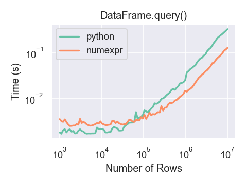
DataFrame.query() で numexpr エンジンを使用するパフォーマンス上のメリットは、フレームが約100,000行を超える場合にのみ見られます。
このプロットは、それぞれ numpy.random.randn() を使用して生成された浮動小数点値を含む3つの列を持つ DataFrame を使用して作成されました。
In [296]: df = pd.DataFrame(np.random.randn(8, 4),
   .....:                   index=dates, columns=['A', 'B', 'C', 'D'])
   .....:

In [297]: df2 = df.copy()
重複データ#
DataFrame内の重複する行を特定して削除したい場合、duplicated と drop_duplicates の2つのメソッドが役立ちます。それぞれ、重複する行を特定するために使用する列を引数として取ります。
duplicatedは、行数と同じ長さのブールベクトルを返し、行が重複しているかどうかを示します。drop_duplicatesは重複する行を削除します。
デフォルトでは、重複するセットの最初の行がユニークと見なされますが、各メソッドには保持するターゲットを指定する keep パラメータがあります。
keep='first'(デフォルト): 最初の出現を除く重複をマーク/削除します。keep='last': 最後の出現を除く重複をマーク/削除します。keep=False: すべての重複をマーク/削除します。
In [298]: df2 = pd.DataFrame({'a': ['one', 'one', 'two', 'two', 'two', 'three', 'four'],
   .....:                     'b': ['x', 'y', 'x', 'y', 'x', 'x', 'x'],
   .....:                     'c': np.random.randn(7)})
   .....:

In [299]: df2
Out[299]:
       a  b         c
0    one  x -1.067137
1    one  y  0.309500
2    two  x -0.211056
3    two  y -1.842023
4    two  x -0.390820
5  three  x -1.964475
6   four  x  1.298329

In [300]: df2.duplicated('a')
Out[300]:
0    False
1     True
2    False
3     True
4     True
5    False
6    False
dtype: bool

In [301]: df2.duplicated('a', keep='last')
Out[301]:
0     True
1    False
2     True
3     True
4    False
5    False
6    False
dtype: bool

In [302]: df2.duplicated('a', keep=False)
Out[302]:
0     True
1     True
2     True
3     True
4     True
5    False
6    False
dtype: bool

In [303]: df2.drop_duplicates('a')
Out[303]:
       a  b         c
0    one  x -1.067137
2    two  x -0.211056
5  three  x -1.964475
6   four  x  1.298329

In [304]: df2.drop_duplicates('a', keep='last')
Out[304]:
       a  b         c
1    one  y  0.309500
4    two  x -0.390820
5  three  x -1.964475
6   four  x  1.298329

In [305]: df2.drop_duplicates('a', keep=False)
Out[305]:
       a  b         c
5  three  x -1.964475
6   four  x  1.298329
また、重複を識別するために列のリストを渡すこともできます。
In [306]: df2.duplicated(['a', 'b'])
Out[306]:
0    False
1    False
2    False
3    False
4     True
5    False
6    False
dtype: bool

In [307]: df2.drop_duplicates(['a', 'b'])
Out[307]:
       a  b         c
0    one  x -1.067137
1    one  y  0.309500
2    two  x -0.211056
3    two  y -1.842023
5  three  x -1.964475
6   four  x  1.298329
インデックス値による重複を削除するには、Index.duplicated を使用し、次にスライスを実行します。keep パラメータには同じオプションセットが利用可能です。
In [308]: df3 = pd.DataFrame({'a': np.arange(6),
   .....:                     'b': np.random.randn(6)},
   .....:                    index=['a', 'a', 'b', 'c', 'b', 'a'])
   .....:

In [309]: df3
Out[309]:
   a         b
a  0  1.440455
a  1  2.456086
b  2  1.038402
c  3 -0.894409
b  4  0.683536
a  5  3.082764

In [310]: df3.index.duplicated()
Out[310]: array([False,  True, False, False,  True,  True])

In [311]: df3[~df3.index.duplicated()]
Out[311]:
   a         b
a  0  1.440455
b  2  1.038402
c  3 -0.894409

In [312]: df3[~df3.index.duplicated(keep='last')]
Out[312]:
   a         b
c  3 -0.894409
b  4  0.683536
a  5  3.082764

In [313]: df3[~df3.index.duplicated(keep=False)]
Out[313]:
   a         b
c  3 -0.894409
辞書ライクな get() メソッド#
SeriesとDataFrameのそれぞれに、デフォルト値を返すことができる get メソッドがあります。
In [314]: s = pd.Series([1, 2, 3], index=['a', 'b', 'c'])

In [315]: s.get('a')  # equivalent to s['a']
Out[315]: 1

In [316]: s.get('x', default=-1)
Out[316]: -1
インデックス/列ラベルによる値の検索#
行ラベルと列ラベルのシーケンスが与えられたときに値のセットを抽出したい場合があります。これは pandas.factorize とNumPyインデックス付けで実現できます。例えば
In [317]: df = pd.DataFrame({'col': ["A", "A", "B", "B"],
   .....:                    'A': [80, 23, np.nan, 22],
   .....:                    'B': [80, 55, 76, 67]})
   .....:

In [318]: df
Out[318]:
  col     A   B
0   A  80.0  80
1   A  23.0  55
2   B   NaN  76
3   B  22.0  67

In [319]: idx, cols = pd.factorize(df['col'])

In [320]: df.reindex(cols, axis=1).to_numpy()[np.arange(len(df)), idx]
Out[320]: array([80., 23., 76., 67.])
以前は、これは専用の DataFrame.lookup メソッドで実現できましたが、これはバージョン1.2.0で非推奨となり、バージョン2.0.0で削除されました。
インデックスオブジェクト#
pandas Index クラスとそのサブクラスは、順序付きマルチセット を実装していると見なすことができます。重複は許可されます。
Index は、ルックアップ、データアライメント、再インデックス付けに必要なインフラストラクチャも提供します。Index を直接作成する最も簡単な方法は、list または他のシーケンスを Index に渡すことです。
In [321]: index = pd.Index(['e', 'd', 'a', 'b'])

In [322]: index
Out[322]: Index(['e', 'd', 'a', 'b'], dtype='object')

In [323]: 'd' in index
Out[323]: True
または数字を使用します
In [324]: index = pd.Index([1, 5, 12])

In [325]: index
Out[325]: Index([1, 5, 12], dtype='int64')

In [326]: 5 in index
Out[326]: True
dtypeが指定されていない場合、Index はデータからdtypeを推測しようとします。Index をインスタンス化する際に明示的なdtypeを与えることも可能です。
In [327]: index = pd.Index(['e', 'd', 'a', 'b'], dtype="string")

In [328]: index
Out[328]: Index(['e', 'd', 'a', 'b'], dtype='string')

In [329]: index = pd.Index([1, 5, 12], dtype="int8")

In [330]: index
Out[330]: Index([1, 5, 12], dtype='int8')

In [331]: index = pd.Index([1, 5, 12], dtype="float32")

In [332]: index
Out[332]: Index([1.0, 5.0, 12.0], dtype='float32')
インデックスに保存する name を渡すこともできます。
In [333]: index = pd.Index(['e', 'd', 'a', 'b'], name='something')

In [334]: index.name
Out[334]: 'something'
名前が設定されている場合、コンソール表示に表示されます。
In [335]: index = pd.Index(list(range(5)), name='rows')

In [336]: columns = pd.Index(['A', 'B', 'C'], name='cols')

In [337]: df = pd.DataFrame(np.random.randn(5, 3), index=index, columns=columns)

In [338]: df
Out[338]:
cols         A         B         C
rows
0     1.295989 -1.051694  1.340429
1    -2.366110  0.428241  0.387275
2     0.433306  0.929548  0.278094
3     2.154730 -0.315628  0.264223
4     1.126818  1.132290 -0.353310

In [339]: df['A']
Out[339]:
rows
0    1.295989
1   -2.366110
2    0.433306
3    2.154730
4    1.126818
Name: A, dtype: float64
メタデータの設定#
インデックスは「ほとんど変更不可能」ですが、name 属性を設定および変更することは可能です。rename、set_names を使用してこれらの属性を直接設定でき、デフォルトではコピーを返します。
MultiIndexの使用法については、高度なインデックス付け を参照してください。
In [340]: ind = pd.Index([1, 2, 3])

In [341]: ind.rename("apple")
Out[341]: Index([1, 2, 3], dtype='int64', name='apple')

In [342]: ind
Out[342]: Index([1, 2, 3], dtype='int64')

In [343]: ind = ind.set_names(["apple"])

In [344]: ind.name = "bob"

In [345]: ind
Out[345]: Index([1, 2, 3], dtype='int64', name='bob')
set_names、set_levels、および set_codes もオプションの level 引数を受け入れます。
In [346]: index = pd.MultiIndex.from_product([range(3), ['one', 'two']], names=['first', 'second'])

In [347]: index
Out[347]:
MultiIndex([(0, 'one'),
            (0, 'two'),
            (1, 'one'),
            (1, 'two'),
            (2, 'one'),
            (2, 'two')],
           names=['first', 'second'])

In [348]: index.levels[1]
Out[348]: Index(['one', 'two'], dtype='object', name='second')

In [349]: index.set_levels(["a", "b"], level=1)
Out[349]:
MultiIndex([(0, 'a'),
            (0, 'b'),
            (1, 'a'),
            (1, 'b'),
            (2, 'a'),
            (2, 'b')],
           names=['first', 'second'])
Indexオブジェクトに対する集合演算#
2つの主な操作は union と intersection です。.difference() メソッドを介して差分が提供されます。
In [350]: a = pd.Index(['c', 'b', 'a'])

In [351]: b = pd.Index(['c', 'e', 'd'])

In [352]: a.difference(b)
Out[352]: Index(['a', 'b'], dtype='object')
symmetric_difference 演算も利用可能で、これは idx1 または idx2 のいずれかに表示されるが、両方には表示されない要素を返します。これは、重複が削除された idx1.difference(idx2).union(idx2.difference(idx1)) によって作成されたインデックスと同等です。
In [353]: idx1 = pd.Index([1, 2, 3, 4])

In [354]: idx2 = pd.Index([2, 3, 4, 5])

In [355]: idx1.symmetric_difference(idx2)
Out[355]: Index([1, 5], dtype='int64')
注
集合演算から得られるインデックスは昇順にソートされます。
異なるdtypeを持つインデックス間で Index.union() を実行する場合、インデックスは共通のdtypeにキャストされる必要があります。通常、常にではありませんが、これはobject dtypeです。例外は、整数データと浮動小数点データの間でunionを実行する場合です。この場合、整数値は浮動小数点に変換されます。
In [356]: idx1 = pd.Index([0, 1, 2])

In [357]: idx2 = pd.Index([0.5, 1.5])

In [358]: idx1.union(idx2)
Out[358]: Index([0.0, 0.5, 1.0, 1.5, 2.0], dtype='float64')
欠損値#
重要
Index は欠損値(NaN)を保持できますが、予期しない結果を望まない場合は避けるべきです。例えば、一部の操作は欠損値を暗黙的に除外します。
Index.fillna は、欠損値を指定されたスカラ値で埋めます。
In [359]: idx1 = pd.Index([1, np.nan, 3, 4])

In [360]: idx1
Out[360]: Index([1.0, nan, 3.0, 4.0], dtype='float64')

In [361]: idx1.fillna(2)
Out[361]: Index([1.0, 2.0, 3.0, 4.0], dtype='float64')

In [362]: idx2 = pd.DatetimeIndex([pd.Timestamp('2011-01-01'),
   .....:                          pd.NaT,
   .....:                          pd.Timestamp('2011-01-03')])
   .....:

In [363]: idx2
Out[363]: DatetimeIndex(['2011-01-01', 'NaT', '2011-01-03'], dtype='datetime64[ns]', freq=None)

In [364]: idx2.fillna(pd.Timestamp('2011-01-02'))
Out[364]: DatetimeIndex(['2011-01-01', '2011-01-02', '2011-01-03'], dtype='datetime64[ns]', freq=None)
インデックスの設定/リセット#
DataFrameにデータセットを読み込んだり作成したりした後で、インデックスを追加したい場合があります。いくつかの異なる方法があります。
インデックスを設定#
DataFrameには set_index() メソッドがあり、列名(通常の Index の場合)または列名のリスト(MultiIndex の場合)を受け取ります。新しい、再インデックスされたDataFrameを作成するには、
In [365]: data = pd.DataFrame({'a': ['bar', 'bar', 'foo', 'foo'],
   .....:                      'b': ['one', 'two', 'one', 'two'],
   .....:                      'c': ['z', 'y', 'x', 'w'],
   .....:                      'd': [1., 2., 3, 4]})
   .....:

In [366]: data
Out[366]:
     a    b  c    d
0  bar  one  z  1.0
1  bar  two  y  2.0
2  foo  one  x  3.0
3  foo  two  w  4.0

In [367]: indexed1 = data.set_index('c')

In [368]: indexed1
Out[368]:
     a    b    d
c
z  bar  one  1.0
y  bar  two  2.0
x  foo  one  3.0
w  foo  two  4.0

In [369]: indexed2 = data.set_index(['a', 'b'])

In [370]: indexed2
Out[370]:
         c    d
a   b
bar one  z  1.0
    two  y  2.0
foo one  x  3.0
    two  w  4.0
append キーワードオプションを使用すると、既存のインデックスを保持し、指定された列をMultiIndexに追加できます。
In [371]: frame = data.set_index('c', drop=False)

In [372]: frame = frame.set_index(['a', 'b'], append=True)

In [373]: frame
Out[373]:
           c    d
c a   b
z bar one  z  1.0
y bar two  y  2.0
x foo one  x  3.0
w foo two  w  4.0
set_index の他のオプションを使用すると、インデックス列を削除しないことができます。
In [374]: data.set_index('c', drop=False)
Out[374]:
     a    b  c    d
c
z  bar  one  z  1.0
y  bar  two  y  2.0
x  foo  one  x  3.0
w  foo  two  w  4.0
インデックスのリセット#
利便性のために、DataFrameには reset_index() と呼ばれる新しい関数があり、インデックス値をDataFrameの列に転送し、単純な整数インデックスを設定します。これは set_index() の逆操作です。
In [375]: data
Out[375]:
     a    b  c    d
0  bar  one  z  1.0
1  bar  two  y  2.0
2  foo  one  x  3.0
3  foo  two  w  4.0

In [376]: data.reset_index()
Out[376]:
   index    a    b  c    d
0      0  bar  one  z  1.0
1      1  bar  two  y  2.0
2      2  foo  one  x  3.0
3      3  foo  two  w  4.0
出力はSQLテーブルやレコード配列に似ています。インデックスから派生した列の名前は、names 属性に格納されているものです。
level キーワードを使用して、インデックスの一部のみを削除できます。
In [377]: frame
Out[377]:
           c    d
c a   b
z bar one  z  1.0
y bar two  y  2.0
x foo one  x  3.0
w foo two  w  4.0

In [378]: frame.reset_index(level=1)
Out[378]:
         a  c    d
c b
z one  bar  z  1.0
y two  bar  y  2.0
x one  foo  x  3.0
w two  foo  w  4.0
reset_index はオプションのパラメータ drop を受け入れます。これがTrueの場合、インデックス値をDataFrameの列に配置する代わりに、インデックスを単純に破棄します。
アドホックなインデックスの追加#
index 属性にカスタムインデックスを割り当てることができます。
In [379]: df_idx = pd.DataFrame(range(4))

In [380]: df_idx.index = pd.Index([10, 20, 30, 40], name="a")

In [381]: df_idx
Out[381]:
    0
a
10  0
20  1
30  2
40  3
ビューを返すかコピーを返すか#
警告
Copy-on-Write はpandas 3.0で新しいデフォルトになります。これは、チェインインデックスは決して機能しないことを意味します。結果として、SettingWithCopyWarning はもう不要になります。詳細については、このセクション を参照してください。pandas 3.0が利用可能になる前に、以下の設定でCopy-on-Writeを有効にして改善を活用することをお勧めします。
` pd.options.mode.copy_on_write = True `
たとえpandas 3.0がまだ利用可能でなくても。
pandasオブジェクトに値を設定する際、chained indexing と呼ばれるものを避けるために注意が必要です。以下に例を示します。
In [382]: dfmi = pd.DataFrame([list('abcd'),
   .....:                      list('efgh'),
   .....:                      list('ijkl'),
   .....:                      list('mnop')],
   .....:                     columns=pd.MultiIndex.from_product([['one', 'two'],
   .....:                                                         ['first', 'second']]))
   .....:

In [383]: dfmi
Out[383]:
    one          two
  first second first second
0     a      b     c      d
1     e      f     g      h
2     i      j     k      l
3     m      n     o      p
これら2つのアクセス方法を比較してください。
In [384]: dfmi['one']['second']
Out[384]:
0    b
1    f
2    j
3    n
Name: second, dtype: object
In [385]: dfmi.loc[:, ('one', 'second')]
Out[385]:
0    b
1    f
2    j
3    n
Name: (one, second), dtype: object
どちらも同じ結果を生成しますが、どちらを使用すべきでしょうか?これらの操作の順序と、なぜメソッド2(.loc)がメソッド1(連結された [])よりもはるかに好まれるのかを理解することは有益です。
dfmi['one'] は列の最初のレベルを選択し、単一インデックスのDataFrameを返します。次に、別のPython操作 dfmi_with_one['second'] は 'second' でインデックス付けされたSeriesを選択します。これは変数 dfmi_with_one で示されています。なぜなら、pandasはこれらの操作を個別のイベント、つまり __getitem__ への個別の呼び出しとして認識するため、線形操作として扱わなければならず、連続して発生するからです。
これに対し、df.loc[:,('one','second')] は、(slice(None),('one','second')) のネストされたタプルを __getitem__ への単一の呼び出しに渡します。これにより、pandasはこれを単一のエンティティとして扱うことができます。さらに、この操作順序は 大幅に 高速になる可能性があり、必要に応じて 両方の 軸をインデックス付けすることができます。
チェインインデックスを使用すると割り当てが失敗するのはなぜですか?#
警告
Copy-on-Write はpandas 3.0で新しいデフォルトになります。これは、チェインインデックスは決して機能しないことを意味します。結果として、SettingWithCopyWarning はもう不要になります。詳細については、このセクション を参照してください。
` pd.options.mode.copy_on_write = True `
たとえpandas 3.0がまだ利用可能でなくても。
前のセクションの問題は単なるパフォーマンスの問題です。SettingWithCopy 警告はどうなっているのでしょうか?通常、数ミリ秒余計にかかるようなことをしても警告を出すことはありません!
しかし、連鎖インデックス付けの生成物に代入することは、本質的に予測不可能な結果をもたらすことが判明しました。これを見るには、Pythonインタプリタがこのコードをどのように実行するかを考えてみてください。
dfmi.loc[:, ('one', 'second')] = value
# becomes
dfmi.loc.__setitem__((slice(None), ('one', 'second')), value)
しかし、このコードは異なる方法で処理されます。
dfmi['one']['second'] = value
# becomes
dfmi.__getitem__('one').__setitem__('second', value)
そこに __getitem__ があることに気づきましたか?単純なケースを除いて、それがビューを返すかコピーを返すかを予測するのは非常に困難であり(配列のメモリレイアウトに依存しますが、pandasはその保証をしません)、したがって __setitem__ が dfmi を変更するのか、それともすぐに破棄される一時オブジェクトを変更するのかも予測できません。**それが** SettingWithCopy が警告していることです!
注
最初の例の loc プロパティについて心配すべきかどうか疑問に思っているかもしれません。しかし、dfmi.loc は変更されたインデックス付け動作を持つ dfmi 自体であることが保証されているため、dfmi.loc.__getitem__ / dfmi.loc.__setitem__ は dfmi に直接作用します。もちろん、dfmi.loc.__getitem__(idx) は dfmi のビューまたはコピーである可能性があります。
時として、連鎖インデックス付けが明確に行われていないように見える場合でも、SettingWithCopy 警告が発生することがあります。**これら**こそが、SettingWithCopy が捕捉するように設計されたバグです!pandasは、おそらくあなたが次のことをしたと警告しようとしています。
def do_something(df):
    foo = df[['bar', 'baz']]  # Is foo a view? A copy? Nobody knows!
    # ... many lines here ...
    # We don't know whether this will modify df or not!
    foo['quux'] = value
    return foo
おやまあ!
評価順序が重要#
警告
Copy-on-Write はpandas 3.0で新しいデフォルトになります。これは、チェインインデックスは決して機能しないことを意味します。結果として、SettingWithCopyWarning はもう不要になります。詳細については、このセクション を参照してください。
` pd.options.mode.copy_on_write = True `
たとえpandas 3.0がまだ利用可能でなくても。
連鎖インデックス付けを使用する場合、インデックス付け操作の順序とタイプによって、結果が元のオブジェクトへのスライスになるか、スライスのコピーになるかが部分的に決定されます。
pandasには SettingWithCopyWarning があります。なぜなら、スライスのコピーに代入することは意図的ではないことが多く、スライスが期待された場所で連鎖インデックス付けがコピーを返すことによって引き起こされる間違いだからです。
pandasが、連結インデックス式への代入について、より信頼するように、または信頼しないようにするには、オプション mode.chained_assignment を以下のいずれかの値に設定できます。
デフォルトの
'warn'は、SettingWithCopyWarningが出力されることを意味します。'raise'は、pandasが対処しなければならないSettingWithCopyErrorを発生させることを意味します。Noneは、警告を完全に抑制します。
In [386]: dfb = pd.DataFrame({'a': ['one', 'one', 'two',
   .....:                           'three', 'two', 'one', 'six'],
   .....:                     'c': np.arange(7)})
   .....:

# This will show the SettingWithCopyWarning
# but the frame values will be set
In [387]: dfb['c'][dfb['a'].str.startswith('o')] = 42
ただし、これはコピーに対して操作を行っているため、機能しません。
In [388]: with pd.option_context('mode.chained_assignment','warn'):
   .....:     dfb[dfb['a'].str.startswith('o')]['c'] = 42
   .....:
連鎖代入は、混合dtypeフレームでの設定でも発生する可能性があります。
注
これらの設定ルールは、.loc/.ilocのすべてに適用されます。
以下は、複数のアイテムに対して(maskを使用して).locを使用し、固定インデックスを使用して単一のアイテムにアクセスするための推奨される方法です。
In [389]: dfc = pd.DataFrame({'a': ['one', 'one', 'two',
   .....:                           'three', 'two', 'one', 'six'],
   .....:                     'c': np.arange(7)})
   .....:

In [390]: dfd = dfc.copy()

# Setting multiple items using a mask
In [391]: mask = dfd['a'].str.startswith('o')

In [392]: dfd.loc[mask, 'c'] = 42

In [393]: dfd
Out[393]:
       a   c
0    one  42
1    one  42
2    two   2
3  three   3
4    two   4
5    one  42
6    six   6

# Setting a single item
In [394]: dfd = dfc.copy()

In [395]: dfd.loc[2, 'a'] = 11

In [396]: dfd
Out[396]:
       a  c
0    one  0
1    one  1
2     11  2
3  three  3
4    two  4
5    one  5
6    six  6
以下は時に機能することもありますが、保証されていないため、避けるべきです。
In [397]: dfd = dfc.copy()

In [398]: dfd['a'][2] = 111

In [399]: dfd
Out[399]:
       a  c
0    one  0
1    one  1
2    111  2
3  three  3
4    two  4
5    one  5
6    six  6
最後に、続く例はまったく機能しないため、避けるべきです。
In [400]: with pd.option_context('mode.chained_assignment','raise'):
   .....:     dfd.loc[0]['a'] = 1111
   .....:
---------------------------------------------------------------------------
SettingWithCopyError                      Traceback (most recent call last)
<ipython-input-400-32ce785aaa5b> in ?()
      1 with pd.option_context('mode.chained_assignment','raise'):
----> 2     dfd.loc[0]['a'] = 1111

~/work/pandas/pandas/pandas/core/series.py in ?(self, key, value)
   1293                 )
   1294
   1295         check_dict_or_set_indexers(key)
   1296         key = com.apply_if_callable(key, self)
-> 1297         cacher_needs_updating = self._check_is_chained_assignment_possible()
   1298
   1299         if key is Ellipsis:
   1300             key = slice(None)

~/work/pandas/pandas/pandas/core/series.py in ?(self)
   1498             ref = self._get_cacher()
   1499             if ref is not None and ref._is_mixed_type:
   1500                 self._check_setitem_copy(t="referent", force=True)
   1501             return True
-> 1502         return super()._check_is_chained_assignment_possible()

~/work/pandas/pandas/pandas/core/generic.py in ?(self)
   4414         single-dtype meaning that the cacher should be updated following
   4415         setting.
   4416         """
   4417         if self._is_copy:
-> 4418             self._check_setitem_copy(t="referent")
   4419         return False

~/work/pandas/pandas/pandas/core/generic.py in ?(self, t, force)
   4488                 "indexing.html#returning-a-view-versus-a-copy"
   4489             )
   4490
   4491         if value == "raise":
-> 4492             raise SettingWithCopyError(t)
   4493         if value == "warn":
   4494             warnings.warn(t, SettingWithCopyWarning, stacklevel=find_stack_level())

SettingWithCopyError:
A value is trying to be set on a copy of a slice from a DataFrame

See the caveats in the documentation: https://pandas.dokyumento.jp/pandas-docs/stable/user_guide/indexing.html#returning-a-view-versus-a-copy
警告
連鎖代入の警告/例外は、ユーザーに無効な代入の可能性を知らせることを目的としています。誤検知、つまり連鎖代入が誤って報告される状況があるかもしれません。