グループ化：分割・適用・結合#

「グループ化」とは、以下のステップの1つ以上を含むプロセスを指します。

分割：ある基準に基づいてデータをグループに分割します。
適用：各グループに独立して関数を適用します。
結合：結果をデータ構造にまとめます。

このうち、分割ステップは最も単純です。適用ステップでは、次のいずれかの操作を行う場合があります。

集約：各グループの集計統計量（または統計量）を計算します。いくつかの例：
- グループの合計または平均を計算します。
- グループサイズ/カウントを計算します。
変換：グループ固有の計算を実行し、同様のインデックスを持つオブジェクトを返します。いくつかの例：
- グループ内のデータを標準化（zスコア）します。
- 各グループから導出された値を使用して、グループ内のNAを埋めます。
フィルタリング：グループごとの計算がTrueまたはFalseと評価されることに基づいて、一部のグループを破棄します。いくつかの例：
- メンバーが少数のグループに属するデータを破棄します。
- グループの合計または平均に基づいてデータをフィルタリングします。

これらの操作の多くは、GroupByオブジェクトで定義されています。これらの操作は、集約API、ウィンドウAPI、およびリサンプリングAPIの操作と似ています。

特定の操作がこれらのカテゴリのいずれにも該当しない場合、またはこれらのカテゴリの組み合わせである場合があります。そのような場合は、GroupByのapplyメソッドを使用して操作を計算できる場合があります。このメソッドは、適用ステップの結果を調べ、上記の3つのカテゴリのいずれにも当てはまらない場合、それらを1つの結果に適切に結合しようとします。

注記

組み込みのGroupBy操作を使用して複数のステップに分割された操作は、ユーザー定義のPython関数を使用してapplyメソッドを使用するよりも効率的です。

SQLベースのツール（またはitertools）を使用したことがある人にとって、GroupByという名前は非常になじみ深いものです。そのようなツールでは、次のようなコードを書くことができます。

SELECT Column1, Column2, mean(Column3), sum(Column4)
FROM SomeTable
GROUP BY Column1, Column2

pandasでは、このような操作を自然で簡単に表現することを目指しています。GroupBy機能の各領域について説明し、次にいくつかの非自明な例/ユースケースを示します。

詳細な戦略については、クックブックを参照してください。

オブジェクトのグループへの分割#

グループ化の抽象的な定義とは、ラベルとグループ名とのマッピングを提供することです。GroupByオブジェクトを作成するには（GroupByオブジェクトの詳細については後述）、次の操作を実行できます。

In [1]: speeds = pd.DataFrame(
   ...:     [
   ...:         ("bird", "Falconiformes", 389.0),
   ...:         ("bird", "Psittaciformes", 24.0),
   ...:         ("mammal", "Carnivora", 80.2),
   ...:         ("mammal", "Primates", np.nan),
   ...:         ("mammal", "Carnivora", 58),
   ...:     ],
   ...:     index=["falcon", "parrot", "lion", "monkey", "leopard"],
   ...:     columns=("class", "order", "max_speed"),
   ...: )
   ...: 

In [2]: speeds
Out[2]: 
          class           order  max_speed
falcon     bird   Falconiformes      389.0
parrot     bird  Psittaciformes       24.0
lion     mammal       Carnivora       80.2
monkey   mammal        Primates        NaN
leopard  mammal       Carnivora       58.0

In [3]: grouped = speeds.groupby("class")

In [4]: grouped = speeds.groupby(["class", "order"])

マッピングは、さまざまな方法で指定できます。

各インデックスラベルに対して呼び出されるPython関数。
インデックスと同じ長さのリストまたはNumPy配列。
label -> group nameマッピングを提供する辞書またはSeries。
DataFrameオブジェクトの場合、グループ化に使用される列名またはインデックスレベル名を指定する文字列。
上記のいずれかのもののリスト。

これらをまとめてキーと呼びます。たとえば、次のDataFrameを考えてみましょう。

注記

groupbyに渡された文字列は、列またはインデックスレベルのいずれかを指す場合があります。文字列が列名とインデックスレベル名の両方に一致する場合、ValueErrorが発生します。

In [5]: df = pd.DataFrame(
   ...:     {
   ...:         "A": ["foo", "bar", "foo", "bar", "foo", "bar", "foo", "foo"],
   ...:         "B": ["one", "one", "two", "three", "two", "two", "one", "three"],
   ...:         "C": np.random.randn(8),
   ...:         "D": np.random.randn(8),
   ...:     }
   ...: )
   ...: 

In [6]: df
Out[6]: 
     A      B         C         D
0  foo    one  0.469112 -0.861849
1  bar    one -0.282863 -2.104569
2  foo    two -1.509059 -0.494929
3  bar  three -1.135632  1.071804
4  foo    two  1.212112  0.721555
5  bar    two -0.173215 -0.706771
6  foo    one  0.119209 -1.039575
7  foo  three -1.044236  0.271860

DataFrameでは、groupby()を呼び出すことで、GroupByオブジェクトを取得します。このメソッドはpandas.api.typing.DataFrameGroupByインスタンスを返します。A列またはB列、あるいはその両方でグループ化できます。

In [7]: grouped = df.groupby("A")

In [8]: grouped = df.groupby("B")

In [9]: grouped = df.groupby(["A", "B"])

注記

df.groupby('A')はdf.groupby(df['A'])の構文糖です。

列AとBにMultiIndexがある場合、指定した列を除くすべての列でグループ化できます。

In [10]: df2 = df.set_index(["A", "B"])

In [11]: grouped = df2.groupby(level=df2.index.names.difference(["B"]))

In [12]: grouped.sum()
Out[12]: 
            C         D
A                      
bar -1.591710 -1.739537
foo -0.752861 -1.402938

上記のGroupByは、DataFrameをインデックス（行）で分割します。列で分割するには、最初に転置します。

In [13]: def get_letter_type(letter):
   ....:     if letter.lower() in 'aeiou':
   ....:         return 'vowel'
   ....:     else:
   ....:         return 'consonant'
   ....: 

In [14]: grouped = df.T.groupby(get_letter_type)

pandasのIndexオブジェクトは、重複値をサポートしています。groupby操作でグループキーとして一意でないインデックスが使用されている場合、同じインデックス値のすべての値は1つのグループに含まれていると見なされ、したがって集約関数の出力には一意のインデックス値のみが含まれます。

In [15]: index = [1, 2, 3, 1, 2, 3]

In [16]: s = pd.Series([1, 2, 3, 10, 20, 30], index=index)

In [17]: s
Out[17]: 
1     1
2     2
3     3
1    10
2    20
3    30
dtype: int64

In [18]: grouped = s.groupby(level=0)

In [19]: grouped.first()
Out[19]: 
1    1
2    2
3    3
dtype: int64

In [20]: grouped.last()
Out[20]: 
1    10
2    20
3    30
dtype: int64

In [21]: grouped.sum()
Out[21]: 
1    11
2    22
3    33
dtype: int64

必要な場合まで、分割は行われません。GroupByオブジェクトを作成するのは、有効なマッピングを渡したことを確認するためだけです。

注記

複雑なデータ操作の多くは、GroupBy操作で表現できます（ただし、最も効率的な実装であるとは限りません）。ラベルマッピング関数で非常に創造的になることができます。

GroupByのソート#

デフォルトでは、groupby操作中にグループキーがソートされます。ただし、潜在的な高速化のためにsort=Falseを渡すことができます。sort=Falseの場合、グループキー間の順序は、元のDataFrame内のキーの出現順序に従います。

In [22]: df2 = pd.DataFrame({"X": ["B", "B", "A", "A"], "Y": [1, 2, 3, 4]})

In [23]: df2.groupby(["X"]).sum()
Out[23]: 
   Y
X   
A  7
B  3

In [24]: df2.groupby(["X"], sort=False).sum()
Out[24]: 
   Y
X   
B  3
A  7

各グループ内でソートされている観測値の順序は、groupby()によって保持されることに注意してください。たとえば、以下のgroupby()によって作成されたグループは、元のDataFrameに出現した順序です。

In [25]: df3 = pd.DataFrame({"X": ["A", "B", "A", "B"], "Y": [1, 4, 3, 2]})

In [26]: df3.groupby("X").get_group("A")
Out[26]: 
   X  Y
0  A  1
2  A  3

In [27]: df3.groupby(["X"]).get_group(("B",))
Out[27]: 
   X  Y
1  B  4
3  B  2

GroupBy dropna#

デフォルトでは、groupby操作中に、NA値はグループキーから除外されます。ただし、グループキーにNA値を含める場合は、dropna=Falseを渡して実現できます。

In [28]: df_list = [[1, 2, 3], [1, None, 4], [2, 1, 3], [1, 2, 2]]

In [29]: df_dropna = pd.DataFrame(df_list, columns=["a", "b", "c"])

In [30]: df_dropna
Out[30]: 
   a    b  c
0  1  2.0  3
1  1  NaN  4
2  2  1.0  3
3  1  2.0  2

# Default ``dropna`` is set to True, which will exclude NaNs in keys
In [31]: df_dropna.groupby(by=["b"], dropna=True).sum()
Out[31]: 
     a  c
b        
1.0  2  3
2.0  2  5

# In order to allow NaN in keys, set ``dropna`` to False
In [32]: df_dropna.groupby(by=["b"], dropna=False).sum()
Out[32]: 
     a  c
b        
1.0  2  3
2.0  2  5
NaN  1  4

dropna引数のデフォルト設定はTrueであり、これはNAがグループキーに含まれないことを意味します。

GroupByオブジェクトの属性#

groups属性は、キーが計算された一意のグループであり、対応する値が各グループに属する軸ラベルである辞書です。上記の例では、次のようになります。

In [33]: df.groupby("A").groups
Out[33]: {'bar': [1, 3, 5], 'foo': [0, 2, 4, 6, 7]}

In [34]: df.T.groupby(get_letter_type).groups
Out[34]: {'consonant': ['B', 'C', 'D'], 'vowel': ['A']}

GroupByオブジェクトに対して標準的なPythonのlen関数を呼び出すと、グループの数（groups辞書の要素数と同じ）が返されます。

In [35]: grouped = df.groupby(["A", "B"])

In [36]: grouped.groups
Out[36]: {('bar', 'one'): [1], ('bar', 'three'): [3], ('bar', 'two'): [5], ('foo', 'one'): [0, 6], ('foo', 'three'): [7], ('foo', 'two'): [2, 4]}

In [37]: len(grouped)
Out[37]: 6

GroupByは、列名、GroupBy操作、その他の属性をタブ補完します。

In [38]: n = 10

In [39]: weight = np.random.normal(166, 20, size=n)

In [40]: height = np.random.normal(60, 10, size=n)

In [41]: time = pd.date_range("1/1/2000", periods=n)

In [42]: gender = np.random.choice(["male", "female"], size=n)

In [43]: df = pd.DataFrame(
   ....:     {"height": height, "weight": weight, "gender": gender}, index=time
   ....: )
   ....: 

In [44]: df
Out[44]: 
               height      weight  gender
2000-01-01  42.849980  157.500553    male
2000-01-02  49.607315  177.340407    male
2000-01-03  56.293531  171.524640    male
2000-01-04  48.421077  144.251986  female
2000-01-05  46.556882  152.526206    male
2000-01-06  68.448851  168.272968  female
2000-01-07  70.757698  136.431469    male
2000-01-08  58.909500  176.499753  female
2000-01-09  76.435631  174.094104  female
2000-01-10  45.306120  177.540920    male

In [45]: gb = df.groupby("gender")

In [46]: gb.<TAB>  # noqa: E225, E999
gb.agg        gb.boxplot    gb.cummin     gb.describe   gb.filter     gb.get_group  gb.height     gb.last       gb.median     gb.ngroups    gb.plot       gb.rank       gb.std        gb.transform
gb.aggregate  gb.count      gb.cumprod    gb.dtype      gb.first      gb.groups     gb.hist       gb.max        gb.min        gb.nth        gb.prod       gb.resample   gb.sum        gb.var
gb.apply      gb.cummax     gb.cumsum     gb.fillna     gb.gender     gb.head       gb.indices    gb.mean       gb.name       gb.ohlc       gb.quantile   gb.size       gb.tail       gb.weight

MultiIndexを使用したGroupBy#

階層的にインデックス付けされたデータでは、階層のレベルの1つでグループ化するのが自然です。

2レベルのMultiIndexを持つSeriesを作成してみましょう。

In [47]: arrays = [
   ....:     ["bar", "bar", "baz", "baz", "foo", "foo", "qux", "qux"],
   ....:     ["one", "two", "one", "two", "one", "two", "one", "two"],
   ....: ]
   ....: 

In [48]: index = pd.MultiIndex.from_arrays(arrays, names=["first", "second"])

In [49]: s = pd.Series(np.random.randn(8), index=index)

In [50]: s
Out[50]: 
first  second
bar    one      -0.919854
       two      -0.042379
baz    one       1.247642
       two      -0.009920
foo    one       0.290213
       two       0.495767
qux    one       0.362949
       two       1.548106
dtype: float64

次に、sのレベルの1つでグループ化できます。

In [51]: grouped = s.groupby(level=0)

In [52]: grouped.sum()
Out[52]: 
first
bar   -0.962232
baz    1.237723
foo    0.785980
qux    1.911055
dtype: float64

MultiIndexに名前が指定されている場合、レベル番号の代わりにこれらの名前を渡すことができます。

In [53]: s.groupby(level="second").sum()
Out[53]: 
second
one    0.980950
two    1.991575
dtype: float64

複数のレベルでのグループ化がサポートされています。

In [54]: arrays = [
   ....:     ["bar", "bar", "baz", "baz", "foo", "foo", "qux", "qux"],
   ....:     ["doo", "doo", "bee", "bee", "bop", "bop", "bop", "bop"],
   ....:     ["one", "two", "one", "two", "one", "two", "one", "two"],
   ....: ]
   ....: 

In [55]: index = pd.MultiIndex.from_arrays(arrays, names=["first", "second", "third"])

In [56]: s = pd.Series(np.random.randn(8), index=index)

In [57]: s
Out[57]: 
first  second  third
bar    doo     one     -1.131345
               two     -0.089329
baz    bee     one      0.337863
               two     -0.945867
foo    bop     one     -0.932132
               two      1.956030
qux    bop     one      0.017587
               two     -0.016692
dtype: float64

In [58]: s.groupby(level=["first", "second"]).sum()
Out[58]: 
first  second
bar    doo      -1.220674
baz    bee      -0.608004
foo    bop       1.023898
qux    bop       0.000895
dtype: float64

インデックスレベル名はキーとして指定できます。

In [59]: s.groupby(["first", "second"]).sum()
Out[59]: 
first  second
bar    doo      -1.220674
baz    bee      -0.608004
foo    bop       1.023898
qux    bop       0.000895
dtype: float64

sum関数と集約の詳細については後述します。

インデックスレベルと列によるDataFrameのグループ化#

DataFrameは、列とインデックスレベルの組み合わせでグループ化できます。列名とインデックス名の両方、またはGrouperを使用できます。

最初に、MultiIndexを持つDataFrameを作成しましょう。

In [60]: arrays = [
   ....:     ["bar", "bar", "baz", "baz", "foo", "foo", "qux", "qux"],
   ....:     ["one", "two", "one", "two", "one", "two", "one", "two"],
   ....: ]
   ....: 

In [61]: index = pd.MultiIndex.from_arrays(arrays, names=["first", "second"])

In [62]: df = pd.DataFrame({"A": [1, 1, 1, 1, 2, 2, 3, 3], "B": np.arange(8)}, index=index)

In [63]: df
Out[63]: 
              A  B
first second      
bar   one     1  0
      two     1  1
baz   one     1  2
      two     1  3
foo   one     2  4
      two     2  5
qux   one     3  6
      two     3  7

次に、dfを2番目のインデックスレベルとA列でグループ化します。

In [64]: df.groupby([pd.Grouper(level=1), "A"]).sum()
Out[64]: 
          B
second A   
one    1  2
       2  4
       3  6
two    1  4
       2  5
       3  7

インデックスレベルは名前で指定することもできます。

In [65]: df.groupby([pd.Grouper(level="second"), "A"]).sum()
Out[65]: 
          B
second A   
one    1  2
       2  4
       3  6
two    1  4
       2  5
       3  7

インデックスレベル名は、groupbyに直接キーとして指定できます。

In [66]: df.groupby(["second", "A"]).sum()
Out[66]: 
          B
second A   
one    1  2
       2  4
       3  6
two    1  4
       2  5
       3  7

GroupByにおけるDataFrame列の選択#

DataFrameからGroupByオブジェクトを作成したら、各列に対して異なる操作を行いたい場合があります。そのため、DataFrameから列を取得する場合と同様に、GroupByオブジェクトに[]を使用することで、次のことができます。

In [67]: df = pd.DataFrame(
   ....:     {
   ....:         "A": ["foo", "bar", "foo", "bar", "foo", "bar", "foo", "foo"],
   ....:         "B": ["one", "one", "two", "three", "two", "two", "one", "three"],
   ....:         "C": np.random.randn(8),
   ....:         "D": np.random.randn(8),
   ....:     }
   ....: )
   ....: 

In [68]: df
Out[68]: 
     A      B         C         D
0  foo    one -0.575247  1.346061
1  bar    one  0.254161  1.511763
2  foo    two -1.143704  1.627081
3  bar  three  0.215897 -0.990582
4  foo    two  1.193555 -0.441652
5  bar    two -0.077118  1.211526
6  foo    one -0.408530  0.268520
7  foo  three -0.862495  0.024580

In [69]: grouped = df.groupby(["A"])

In [70]: grouped_C = grouped["C"]

In [71]: grouped_D = grouped["D"]

これは主に、より冗長な代替方法に対する構文糖です。

In [72]: df["C"].groupby(df["A"])
Out[72]: <pandas.core.groupby.generic.SeriesGroupBy object at 0x7fac68da1630>

さらに、この方法は、渡されたキーから導出された内部グループ化情報を再計算するのを回避します。

操作対象に含めたい場合は、グループ化列を含めることもできます。

In [73]: grouped[["A", "B"]].sum()
Out[73]: 
                   A                  B
A                                      
bar        barbarbar        onethreetwo
foo  foofoofoofoofoo  onetwotwoonethree

グループの反復処理#

GroupByオブジェクトがあれば、グループ化されたデータの反復処理は非常に自然で、itertools.groupby()と同様に機能します。

In [74]: grouped = df.groupby('A')

In [75]: for name, group in grouped:
   ....:     print(name)
   ....:     print(group)
   ....: 
bar
     A      B         C         D
1  bar    one  0.254161  1.511763
3  bar  three  0.215897 -0.990582
5  bar    two -0.077118  1.211526
foo
     A      B         C         D
0  foo    one -0.575247  1.346061
2  foo    two -1.143704  1.627081
4  foo    two  1.193555 -0.441652
6  foo    one -0.408530  0.268520
7  foo  three -0.862495  0.024580

複数のキーでグループ化する場合、グループ名はタプルになります。

In [76]: for name, group in df.groupby(['A', 'B']):
   ....:     print(name)
   ....:     print(group)
   ....: 
('bar', 'one')
     A    B         C         D
1  bar  one  0.254161  1.511763
('bar', 'three')
     A      B         C         D
3  bar  three  0.215897 -0.990582
('bar', 'two')
     A    B         C         D
5  bar  two -0.077118  1.211526
('foo', 'one')
     A    B         C         D
0  foo  one -0.575247  1.346061
6  foo  one -0.408530  0.268520
('foo', 'three')
     A      B         C        D
7  foo  three -0.862495  0.02458
('foo', 'two')
     A    B         C         D
2  foo  two -1.143704  1.627081
4  foo  two  1.193555 -0.441652

グループの反復処理を参照してください。

グループの選択#

DataFrameGroupBy.get_group()を使用して、単一のグループを選択できます。

In [77]: grouped.get_group("bar")
Out[77]: 
     A      B         C         D
1  bar    one  0.254161  1.511763
3  bar  three  0.215897 -0.990582
5  bar    two -0.077118  1.211526

または、複数の列でグループ化されたオブジェクトの場合

In [78]: df.groupby(["A", "B"]).get_group(("bar", "one"))
Out[78]: 
     A    B         C         D
1  bar  one  0.254161  1.511763

集約#

集約とは、グループ化オブジェクトの次元を削減するGroupBy操作です。集約の結果は、グループ内の各列に対してスカラー値として扱われます。たとえば、値のグループ内の各列の合計を生成します。

In [79]: animals = pd.DataFrame(
   ....:     {
   ....:         "kind": ["cat", "dog", "cat", "dog"],
   ....:         "height": [9.1, 6.0, 9.5, 34.0],
   ....:         "weight": [7.9, 7.5, 9.9, 198.0],
   ....:     }
   ....: )
   ....: 

In [80]: animals
Out[80]: 
  kind  height  weight
0  cat     9.1     7.9
1  dog     6.0     7.5
2  cat     9.5     9.9
3  dog    34.0   198.0

In [81]: animals.groupby("kind").sum()
Out[81]: 
      height  weight
kind                
cat     18.6    17.8
dog     40.0   205.5

結果では、デフォルトでグループのキーがインデックスに表示されます。as_index=Falseを渡すことで、列に含めることができます。

In [82]: animals.groupby("kind", as_index=False).sum()
Out[82]: 
  kind  height  weight
0  cat    18.6    17.8
1  dog    40.0   205.5

組み込み集約メソッド#

多くの一般的な集約は、GroupByオブジェクトにメソッドとして組み込まれています。以下にリストされているメソッドのうち、*が付いているものは、効率的なGroupBy固有の実装がありません。

メソッド	説明
`any()`	グループ内の値のいずれかが真であるかどうかを計算します。
`all()`	グループ内のすべての値が真であるかどうかを計算します。
`count()`	グループ内の非NA値の数を計算します。
`cov()` *	グループの共分散を計算します。
`first()`	各グループで最初に発生する値を計算します。
`idxmax()`	各グループで最大値のインデックスを計算します。
`idxmin()`	各グループで最小値のインデックスを計算します。
`last()`	各グループで最後に発生する値を計算します。
`max()`	各グループの最大値を計算します。
`mean()`	各グループの平均を計算します。
`median()`	各グループの中央値を計算します。
`min()`	各グループの最小値を計算します。
`nunique()`	各グループの一意の値の数を計算します。
`prod()`	各グループの値の積を計算します。
`quantile()`	各グループの値の指定された分位数を計算します。
`sem()`	各グループの値の平均の標準誤差を計算します。
`size()`	各グループの値の数を計算します。
`skew()` *	各グループの値の歪度を計算します。
`std()`	各グループの値の標準偏差を計算します。
`sum()`	各グループの値の合計を計算します。
`var()`	各グループの値の分散を計算します。

いくつかの例

In [83]: df.groupby("A")[["C", "D"]].max()
Out[83]: 
            C         D
A                      
bar  0.254161  1.511763
foo  1.193555  1.627081

In [84]: df.groupby(["A", "B"]).mean()
Out[84]: 
                  C         D
A   B                        
bar one    0.254161  1.511763
    three  0.215897 -0.990582
    two   -0.077118  1.211526
foo one   -0.491888  0.807291
    three -0.862495  0.024580
    two    0.024925  0.592714

別の集約の例として、各グループのサイズを計算します。これは、GroupByのsizeメソッドに含まれています。インデックスがグループ名で、値が各グループのサイズであるSeriesを返します。

In [85]: grouped = df.groupby(["A", "B"])

In [86]: grouped.size()
Out[86]: 
A    B    
bar  one      1
     three    1
     two      1
foo  one      2
     three    1
     two      2
dtype: int64

DataFrameGroupBy.describe()メソッド自体は縮小器ではありませんが、各グループに関する要約統計量の集まりを簡単に生成するために使用できます。

In [87]: grouped.describe()
Out[87]: 
              C                      ...         D                    
          count      mean       std  ...       50%       75%       max
A   B                                ...                              
bar one     1.0  0.254161       NaN  ...  1.511763  1.511763  1.511763
    three   1.0  0.215897       NaN  ... -0.990582 -0.990582 -0.990582
    two     1.0 -0.077118       NaN  ...  1.211526  1.211526  1.211526
foo one     2.0 -0.491888  0.117887  ...  0.807291  1.076676  1.346061
    three   1.0 -0.862495       NaN  ...  0.024580  0.024580  0.024580
    two     2.0  0.024925  1.652692  ...  0.592714  1.109898  1.627081

[6 rows x 16 columns]

別の集約の例として、各グループの一意の値の数を計算します。これはDataFrameGroupBy.value_counts()関数に似ていますが、一意の値の数だけをカウントします。

In [88]: ll = [['foo', 1], ['foo', 2], ['foo', 2], ['bar', 1], ['bar', 1]]

In [89]: df4 = pd.DataFrame(ll, columns=["A", "B"])

In [90]: df4
Out[90]: 
     A  B
0  foo  1
1  foo  2
2  foo  2
3  bar  1
4  bar  1

In [91]: df4.groupby("A")["B"].nunique()
Out[91]: 
A
bar    1
foo    2
Name: B, dtype: int64

注記

集約関数は、デフォルトのas_index=Trueの場合、集約対象のグループを名前付き列として返し**ません**。グループ化された列は、返されたオブジェクトの**インデックス**になります。

as_index=Falseを渡すと、入力で名前付き**インデックス**または列であるかに関係なく、集約対象のグループが名前付き列として返されます。

`aggregate()`メソッド#

注記

aggregate()メソッドは、多くの異なるタイプの入力を受け入れることができます。このセクションでは、さまざまなGroupByメソッドの文字列エイリアスの使用について詳しく説明します。その他の入力については、以下のセクションで詳しく説明します。

pandasが実装する任意の縮小メソッドは、文字列としてaggregate()に渡すことができます。ユーザーは、短縮形であるaggを使用することをお勧めします。対応するメソッドが呼び出されたかのように動作します。

In [92]: grouped = df.groupby("A")

In [93]: grouped[["C", "D"]].aggregate("sum")
Out[93]: 
            C         D
A                      
bar  0.392940  1.732707
foo -1.796421  2.824590

In [94]: grouped = df.groupby(["A", "B"])

In [95]: grouped.agg("sum")
Out[95]: 
                  C         D
A   B                        
bar one    0.254161  1.511763
    three  0.215897 -0.990582
    two   -0.077118  1.211526
foo one   -0.983776  1.614581
    three -0.862495  0.024580
    two    0.049851  1.185429

集約の結果は、グループ名を新しいインデックスとして持ちます。複数のキーの場合、結果はデフォルトでMultiIndexになります。上記のように、as_indexオプションを使用して変更できます。

In [96]: grouped = df.groupby(["A", "B"], as_index=False)

In [97]: grouped.agg("sum")
Out[97]: 
     A      B         C         D
0  bar    one  0.254161  1.511763
1  bar  three  0.215897 -0.990582
2  bar    two -0.077118  1.211526
3  foo    one -0.983776  1.614581
4  foo  three -0.862495  0.024580
5  foo    two  0.049851  1.185429

In [98]: df.groupby("A", as_index=False)[["C", "D"]].agg("sum")
Out[98]: 
     A         C         D
0  bar  0.392940  1.732707
1  foo -1.796421  2.824590

列名が結果のMultiIndexに格納されているため、DataFrame.reset_index() DataFrame関数を使用して同じ結果を得ることができますが、これにより余分なコピーが作成されます。

In [99]: df.groupby(["A", "B"]).agg("sum").reset_index()
Out[99]: 
     A      B         C         D
0  bar    one  0.254161  1.511763
1  bar  three  0.215897 -0.990582
2  bar    two -0.077118  1.211526
3  foo    one -0.983776  1.614581
4  foo  three -0.862495  0.024580
5  foo    two  0.049851  1.185429

ユーザー定義関数を使用した集約#

ユーザーは、カスタム集約のために独自のユーザー定義関数（UDF）を提供することもできます。

警告

UDFで集約する場合、UDFは提供されたSeriesを変更してはなりません。ユーザー定義関数（UDF）メソッドによる変更の詳細を参照してください。

注記

UDFを使用した集約は、GroupByでpandasの組み込みメソッドを使用するよりもパフォーマンスが低いことがよくあります。複雑な操作を、組み込みメソッドを利用する一連の操作に分割することを検討してください。

In [100]: animals
Out[100]: 
  kind  height  weight
0  cat     9.1     7.9
1  dog     6.0     7.5
2  cat     9.5     9.9
3  dog    34.0   198.0

In [101]: animals.groupby("kind")[["height"]].agg(lambda x: set(x))
Out[101]: 
           height
kind             
cat    {9.1, 9.5}
dog   {34.0, 6.0}

結果のdtypeは、集約関数のdtypeを反映します。異なるグループの結果のdtypeが異なる場合、DataFrameの構築と同様に、共通のdtypeが決定されます。

In [102]: animals.groupby("kind")[["height"]].agg(lambda x: x.astype(int).sum())
Out[102]: 
      height
kind        
cat       18
dog       40

一度に複数の関数を適用する#

グループ化されたSeriesでは、関数の一覧または辞書をSeriesGroupBy.agg()に渡して、DataFrameを出力できます。

In [103]: grouped = df.groupby("A")

In [104]: grouped["C"].agg(["sum", "mean", "std"])
Out[104]: 
          sum      mean       std
A                                
bar  0.392940  0.130980  0.181231
foo -1.796421 -0.359284  0.912265

グループ化されたDataFrameでは、関数の一覧をDataFrameGroupBy.agg()に渡して各列を集約し、階層的な列インデックスを持つ集約結果を生成できます。

In [105]: grouped[["C", "D"]].agg(["sum", "mean", "std"])
Out[105]: 
            C                             D                    
          sum      mean       std       sum      mean       std
A                                                              
bar  0.392940  0.130980  0.181231  1.732707  0.577569  1.366330
foo -1.796421 -0.359284  0.912265  2.824590  0.564918  0.884785

結果の集約には、関数自体が名前として付けられます。名前を変更する必要がある場合は、次のようにSeriesのチェーン操作を追加できます。

In [106]: (
   .....:     grouped["C"]
   .....:     .agg(["sum", "mean", "std"])
   .....:     .rename(columns={"sum": "foo", "mean": "bar", "std": "baz"})
   .....: )
   .....: 
Out[106]: 
          foo       bar       baz
A                                
bar  0.392940  0.130980  0.181231
foo -1.796421 -0.359284  0.912265

グループ化されたDataFrameの場合、同様の方法で名前を変更できます。

In [107]: (
   .....:     grouped[["C", "D"]].agg(["sum", "mean", "std"]).rename(
   .....:         columns={"sum": "foo", "mean": "bar", "std": "baz"}
   .....:     )
   .....: )
   .....: 
Out[107]: 
            C                             D                    
          foo       bar       baz       foo       bar       baz
A                                                              
bar  0.392940  0.130980  0.181231  1.732707  0.577569  1.366330
foo -1.796421 -0.359284  0.912265  2.824590  0.564918  0.884785

注記

一般的に、出力列名は一意である必要がありますが、pandasでは同じ関数（または名前が同じ2つの関数）を同じ列に適用できます。

In [108]: grouped["C"].agg(["sum", "sum"])
Out[108]: 
          sum       sum
A                      
bar  0.392940  0.392940
foo -1.796421 -1.796421

pandasでは、複数のラムダを提供することもできます。この場合、pandasは（名前のない）ラムダ関数の名前を改変し、後続の各ラムダに_<i>を追加します。

In [109]: grouped["C"].agg([lambda x: x.max() - x.min(), lambda x: x.median() - x.mean()])
Out[109]: 
     <lambda_0>  <lambda_1>
A                          
bar    0.331279    0.084917
foo    2.337259   -0.215962

名前付き集約#

列ごとの集計を出力列名を制御してサポートするために、pandasはDataFrameGroupBy.agg()とSeriesGroupBy.agg()で、「名前付き集計」として知られる特別な構文を受け入れます。

キーワードは出力列名です。
値は、最初の要素が選択する列で、2番目の要素はその列に適用する集計であるタプルです。pandasはNamedAgg名前付きタプルを提供し、フィールド['column', 'aggfunc']を使用して引数を明確にします。通常どおり、集計は呼び出し可能オブジェクトまたは文字列エイリアスにすることができます。

In [110]: animals
Out[110]: 
  kind  height  weight
0  cat     9.1     7.9
1  dog     6.0     7.5
2  cat     9.5     9.9
3  dog    34.0   198.0

In [111]: animals.groupby("kind").agg(
   .....:     min_height=pd.NamedAgg(column="height", aggfunc="min"),
   .....:     max_height=pd.NamedAgg(column="height", aggfunc="max"),
   .....:     average_weight=pd.NamedAgg(column="weight", aggfunc="mean"),
   .....: )
   .....: 
Out[111]: 
      min_height  max_height  average_weight
kind                                        
cat          9.1         9.5            8.90
dog          6.0        34.0          102.75

NamedAggは単なるnamedtupleです。プレーンなタプルも許容されます。

In [112]: animals.groupby("kind").agg(
   .....:     min_height=("height", "min"),
   .....:     max_height=("height", "max"),
   .....:     average_weight=("weight", "mean"),
   .....: )
   .....: 
Out[112]: 
      min_height  max_height  average_weight
kind                                        
cat          9.1         9.5            8.90
dog          6.0        34.0          102.75

必要な列名が有効なPythonキーワードでない場合は、辞書を作成し、キーワード引数を展開します。

In [113]: animals.groupby("kind").agg(
   .....:     **{
   .....:         "total weight": pd.NamedAgg(column="weight", aggfunc="sum")
   .....:     }
   .....: )
   .....: 
Out[113]: 
      total weight
kind              
cat           17.8
dog          205.5

名前付き集計を使用する場合、追加のキーワード引数は集計関数に渡されません。(column, aggfunc)のペアのみが**kwargsとして渡される必要があります。集計関数が追加の引数が必要な場合は、functools.partial()を使用して部分的に適用します。

名前付き集計は、Series groupby集計にも有効です。この場合、列の選択はないため、値は単なる関数です。

In [114]: animals.groupby("kind").height.agg(
   .....:     min_height="min",
   .....:     max_height="max",
   .....: )
   .....: 
Out[114]: 
      min_height  max_height
kind                        
cat          9.1         9.5
dog          6.0        34.0

DataFrame列への異なる関数の適用#

aggregateに辞書を渡すことで、DataFrameの列に異なる集計を適用できます。

In [115]: grouped.agg({"C": "sum", "D": lambda x: np.std(x, ddof=1)})
Out[115]: 
            C         D
A                      
bar  0.392940  1.366330
foo -1.796421  0.884785

関数名も文字列にすることができます。文字列を有効にするには、GroupByで実装されている必要があります。

In [116]: grouped.agg({"C": "sum", "D": "std"})
Out[116]: 
            C         D
A                      
bar  0.392940  1.366330
foo -1.796421  0.884785

変換#

変換とは、結果がグループ化されているものと同じインデックスを持つGroupBy操作です。一般的な例としては、cumsum()とdiff()などがあります。

In [117]: speeds
Out[117]: 
          class           order  max_speed
falcon     bird   Falconiformes      389.0
parrot     bird  Psittaciformes       24.0
lion     mammal       Carnivora       80.2
monkey   mammal        Primates        NaN
leopard  mammal       Carnivora       58.0

In [118]: grouped = speeds.groupby("class")["max_speed"]

In [119]: grouped.cumsum()
Out[119]: 
falcon     389.0
parrot     413.0
lion        80.2
monkey       NaN
leopard    138.2
Name: max_speed, dtype: float64

In [120]: grouped.diff()
Out[120]: 
falcon       NaN
parrot    -365.0
lion         NaN
monkey       NaN
leopard      NaN
Name: max_speed, dtype: float64

集計とは異なり、元のオブジェクトを分割するために使用されるグループ化は結果に含まれません。

注記

変換には、結果を分割するために使用されるグループ化が含まれていないため、DataFrame.groupby()とSeries.groupby()のas_indexとsort引数は効果がありません。

変換の一般的な用途は、結果を元のDataFrameに追加することです。

In [121]: result = speeds.copy()

In [122]: result["cumsum"] = grouped.cumsum()

In [123]: result["diff"] = grouped.diff()

In [124]: result
Out[124]: 
          class           order  max_speed  cumsum   diff
falcon     bird   Falconiformes      389.0   389.0    NaN
parrot     bird  Psittaciformes       24.0   413.0 -365.0
lion     mammal       Carnivora       80.2    80.2    NaN
monkey   mammal        Primates        NaN     NaN    NaN
leopard  mammal       Carnivora       58.0   138.2    NaN

組み込み変換メソッド#

GroupByの次のメソッドは変換として機能します。

メソッド	説明
`bfill()`	各グループ内のNA値を後ろから埋めます。
`cumcount()`	各グループ内の累積カウントを計算します。
`cummax()`	各グループ内の累積最大値を計算します。
`cummin()`	各グループ内の累積最小値を計算します。
`cumprod()`	各グループ内の累積積を計算します。
`cumsum()`	各グループ内の累積和を計算します。
`diff()`	各グループ内の隣接する値間の差を計算します。
`ffill()`	各グループ内のNA値を前から埋めます。
`pct_change()`	各グループ内の隣接する値間の変化率を計算します。
`rank()`	各グループ内の各値の順位を計算します。
`shift()`	各グループ内で値を上下にシフトします。

さらに、組み込みの集計メソッドを文字列としてtransform()（次のセクションを参照）に渡すと、結果はグループ全体にブロードキャストされ、変換された結果が生成されます。集計メソッドに効率的な実装がある場合、これもパフォーマンスが向上します。

`transform()`メソッド#

集計メソッドと同様に、transform()メソッドは、前のセクションの組み込み変換メソッドへの文字列エイリアスを受け入れることができます。また、組み込み集計メソッドへの文字列エイリアスも受け入れます。集計メソッドが指定されると、結果はグループ全体にブロードキャストされます。

In [125]: speeds
Out[125]: 
          class           order  max_speed
falcon     bird   Falconiformes      389.0
parrot     bird  Psittaciformes       24.0
lion     mammal       Carnivora       80.2
monkey   mammal        Primates        NaN
leopard  mammal       Carnivora       58.0

In [126]: grouped = speeds.groupby("class")[["max_speed"]]

In [127]: grouped.transform("cumsum")
Out[127]: 
         max_speed
falcon       389.0
parrot       413.0
lion          80.2
monkey         NaN
leopard      138.2

In [128]: grouped.transform("sum")
Out[128]: 
         max_speed
falcon       413.0
parrot       413.0
lion         138.2
monkey       138.2
leopard      138.2

文字列エイリアスに加えて、transform()メソッドは、ユーザー定義関数（UDF）も受け入れることができます。UDFは次の必要があります。

グループチャンクと同じサイズ、またはグループチャンクのサイズにブロードキャスト可能な結果を返す（例：スカラー、grouped.transform(lambda x: x.iloc[-1])）。
グループチャンクで列ごとに操作します。変換は、chunk.applyを使用して最初のグループチャンクに適用されます。
グループチャンクでインプレース操作を実行しません。グループチャンクは不変として扱う必要があり、グループチャンクへの変更は予期しない結果を招く可能性があります。詳細については、ユーザー定義関数（UDF）メソッドによる変更を参照してください。
(オプション)グループチャンク全体のすべての列を一度に操作します。これがサポートされている場合、2番目のチャンクから始まる高速パスが使用されます。

注記

UDFを使用してtransformに供給することで変換を行うと、GroupByの組み込みメソッドを使用する場合よりもパフォーマンスが低下することがよくあります。複雑な操作を、組み込みメソッドを利用する一連の操作に分割することを検討してください。

このセクションのすべての例は、UDFを使用する代わりに組み込みメソッドを呼び出すことで、パフォーマンスを向上させることができます。以下の例を参照してください。

バージョン2.0.0で変更されました：グループ化されたDataFrameで.transformを使用し、変換関数がDataFrameを返す場合、pandasは現在、結果のインデックスを入力値のインデックスと整合させます。変換関数内で.to_numpy()を呼び出すと、整合を回避できます。

aggregate()メソッドと同様に、結果のdtypeは変換関数のdtypeを反映します。異なるグループの結果のdtypeが異なる場合、DataFrameの作成と同じ方法で共通のdtypeが決定されます。

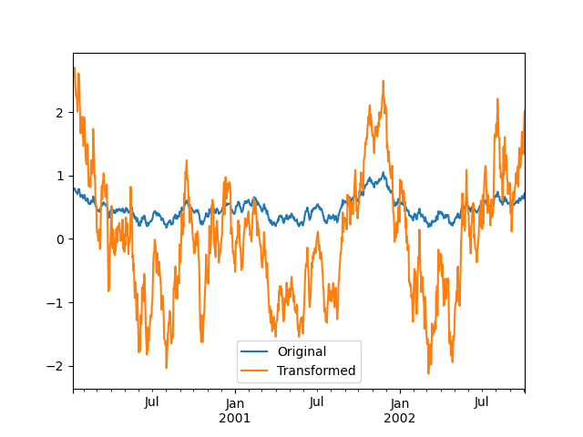
各グループ内のデータを標準化したいとします。

In [129]: index = pd.date_range("10/1/1999", periods=1100)

In [130]: ts = pd.Series(np.random.normal(0.5, 2, 1100), index)

In [131]: ts = ts.rolling(window=100, min_periods=100).mean().dropna()

In [132]: ts.head()
Out[132]: 
2000-01-08    0.779333
2000-01-09    0.778852
2000-01-10    0.786476
2000-01-11    0.782797
2000-01-12    0.798110
Freq: D, dtype: float64

In [133]: ts.tail()
Out[133]: 
2002-09-30    0.660294
2002-10-01    0.631095
2002-10-02    0.673601
2002-10-03    0.709213
2002-10-04    0.719369
Freq: D, dtype: float64

In [134]: transformed = ts.groupby(lambda x: x.year).transform(
   .....:     lambda x: (x - x.mean()) / x.std()
   .....: )
   .....: 

結果は、各グループ内で平均が0、標準偏差が1になることが期待されます（浮動小数点誤差まで）。これは簡単に確認できます。

# Original Data
In [135]: grouped = ts.groupby(lambda x: x.year)

In [136]: grouped.mean()
Out[136]: 
2000    0.442441
2001    0.526246
2002    0.459365
dtype: float64

In [137]: grouped.std()
Out[137]: 
2000    0.131752
2001    0.210945
2002    0.128753
dtype: float64

# Transformed Data
In [138]: grouped_trans = transformed.groupby(lambda x: x.year)

In [139]: grouped_trans.mean()
Out[139]: 
2000   -4.870756e-16
2001   -1.545187e-16
2002    4.136282e-16
dtype: float64

In [140]: grouped_trans.std()
Out[140]: 
2000    1.0
2001    1.0
2002    1.0
dtype: float64

元のデータセットと変換されたデータセットを視覚的に比較することもできます。

In [141]: compare = pd.DataFrame({"Original": ts, "Transformed": transformed})

In [142]: compare.plot()
Out[142]: <Axes: >

次元が低い出力を持つ変換関数は、入力配列の形状に一致するようにブロードキャストされます。

In [143]: ts.groupby(lambda x: x.year).transform(lambda x: x.max() - x.min())
Out[143]: 
2000-01-08    0.623893
2000-01-09    0.623893
2000-01-10    0.623893
2000-01-11    0.623893
2000-01-12    0.623893
                ...   
2002-09-30    0.558275
2002-10-01    0.558275
2002-10-02    0.558275
2002-10-03    0.558275
2002-10-04    0.558275
Freq: D, Length: 1001, dtype: float64

もう1つの一般的なデータ変換は、欠損データをグループ平均で置き換えることです。

In [144]: cols = ["A", "B", "C"]

In [145]: values = np.random.randn(1000, 3)

In [146]: values[np.random.randint(0, 1000, 100), 0] = np.nan

In [147]: values[np.random.randint(0, 1000, 50), 1] = np.nan

In [148]: values[np.random.randint(0, 1000, 200), 2] = np.nan

In [149]: data_df = pd.DataFrame(values, columns=cols)

In [150]: data_df
Out[150]: 
            A         B         C
0    1.539708 -1.166480  0.533026
1    1.302092 -0.505754       NaN
2   -0.371983  1.104803 -0.651520
3   -1.309622  1.118697 -1.161657
4   -1.924296  0.396437  0.812436
..        ...       ...       ...
995 -0.093110  0.683847 -0.774753
996 -0.185043  1.438572       NaN
997 -0.394469 -0.642343  0.011374
998 -1.174126  1.857148       NaN
999  0.234564  0.517098  0.393534

[1000 rows x 3 columns]

In [151]: countries = np.array(["US", "UK", "GR", "JP"])

In [152]: key = countries[np.random.randint(0, 4, 1000)]

In [153]: grouped = data_df.groupby(key)

# Non-NA count in each group
In [154]: grouped.count()
Out[154]: 
      A    B    C
GR  209  217  189
JP  240  255  217
UK  216  231  193
US  239  250  217

In [155]: transformed = grouped.transform(lambda x: x.fillna(x.mean()))

変換されたデータではグループ平均が変わっておらず、変換されたデータにNAが含まれていないことを確認できます。

In [156]: grouped_trans = transformed.groupby(key)

In [157]: grouped.mean()  # original group means
Out[157]: 
           A         B         C
GR -0.098371 -0.015420  0.068053
JP  0.069025  0.023100 -0.077324
UK  0.034069 -0.052580 -0.116525
US  0.058664 -0.020399  0.028603

In [158]: grouped_trans.mean()  # transformation did not change group means
Out[158]: 
           A         B         C
GR -0.098371 -0.015420  0.068053
JP  0.069025  0.023100 -0.077324
UK  0.034069 -0.052580 -0.116525
US  0.058664 -0.020399  0.028603

In [159]: grouped.count()  # original has some missing data points
Out[159]: 
      A    B    C
GR  209  217  189
JP  240  255  217
UK  216  231  193
US  239  250  217

In [160]: grouped_trans.count()  # counts after transformation
Out[160]: 
      A    B    C
GR  228  228  228
JP  267  267  267
UK  247  247  247
US  258  258  258

In [161]: grouped_trans.size()  # Verify non-NA count equals group size
Out[161]: 
GR    228
JP    267
UK    247
US    258
dtype: int64

上記の注記で述べたように、このセクションの各例は、組み込みメソッドを使用してより効率的に計算できます。以下のコードでは、UDFを使用する非効率的な方法はコメントアウトされ、より高速な代替方法が表示されます。

# result = ts.groupby(lambda x: x.year).transform(
#     lambda x: (x - x.mean()) / x.std()
# )
In [162]: grouped = ts.groupby(lambda x: x.year)

In [163]: result = (ts - grouped.transform("mean")) / grouped.transform("std")

# result = ts.groupby(lambda x: x.year).transform(lambda x: x.max() - x.min())
In [164]: grouped = ts.groupby(lambda x: x.year)

In [165]: result = grouped.transform("max") - grouped.transform("min")

# grouped = data_df.groupby(key)
# result = grouped.transform(lambda x: x.fillna(x.mean()))
In [166]: grouped = data_df.groupby(key)

In [167]: result = data_df.fillna(grouped.transform("mean"))

ウィンドウとリサンプリング操作#

resample()、expanding()、rolling()をgroupbyのメソッドとして使用できます。

以下の例では、列Aのグループに基づいて、列Bのサンプルにrolling()メソッドを適用します。

In [168]: df_re = pd.DataFrame({"A": [1] * 10 + [5] * 10, "B": np.arange(20)})

In [169]: df_re
Out[169]: 
    A   B
0   1   0
1   1   1
2   1   2
3   1   3
4   1   4
.. ..  ..
15  5  15
16  5  16
17  5  17
18  5  18
19  5  19

[20 rows x 2 columns]

In [170]: df_re.groupby("A").rolling(4).B.mean()
Out[170]: 
A    
1  0      NaN
   1      NaN
   2      NaN
   3      1.5
   4      2.5
         ... 
5  15    13.5
   16    14.5
   17    15.5
   18    16.5
   19    17.5
Name: B, Length: 20, dtype: float64

expanding()メソッドは、各特定のグループのすべてのメンバーに対して特定の操作（例ではsum()）を累積します。

In [171]: df_re.groupby("A").expanding().sum()
Out[171]: 
          B
A          
1 0     0.0
  1     1.0
  2     3.0
  3     6.0
  4    10.0
...     ...
5 15   75.0
  16   91.0
  17  108.0
  18  126.0
  19  145.0

[20 rows x 1 columns]

DataFrameの各グループで日次頻度を取得するためにresample()メソッドを使用し、欠損値をffill()メソッドで補完したいとします。

In [172]: df_re = pd.DataFrame(
   .....:     {
   .....:         "date": pd.date_range(start="2016-01-01", periods=4, freq="W"),
   .....:         "group": [1, 1, 2, 2],
   .....:         "val": [5, 6, 7, 8],
   .....:     }
   .....: ).set_index("date")
   .....: 

In [173]: df_re
Out[173]: 
            group  val
date                  
2016-01-03      1    5
2016-01-10      1    6
2016-01-17      2    7
2016-01-24      2    8

In [174]: df_re.groupby("group").resample("1D", include_groups=False).ffill()
Out[174]: 
                  val
group date           
1     2016-01-03    5
      2016-01-04    5
      2016-01-05    5
      2016-01-06    5
      2016-01-07    5
...               ...
2     2016-01-20    7
      2016-01-21    7
      2016-01-22    7
      2016-01-23    7
      2016-01-24    8

[16 rows x 1 columns]

フィルタリング#

フィルタリングとは、元のグループ化オブジェクトをサブセット化するGroupBy操作です。グループ全体、グループの一部、またはその両方を取り除くことができます。フィルタリングは、指定された場合にグループ化列を含む、呼び出し元のオブジェクトのフィルタリングされたバージョンを返します。次の例では、classは結果に含まれています。

In [175]: speeds
Out[175]: 
          class           order  max_speed
falcon     bird   Falconiformes      389.0
parrot     bird  Psittaciformes       24.0
lion     mammal       Carnivora       80.2
monkey   mammal        Primates        NaN
leopard  mammal       Carnivora       58.0

In [176]: speeds.groupby("class").nth(1)
Out[176]: 
         class           order  max_speed
parrot    bird  Psittaciformes       24.0
monkey  mammal        Primates        NaN

注記

集計とは異なり、フィルタリングは結果のインデックスにグループキーを追加しません。そのため、as_index=Falseまたはsort=Trueを渡しても、これらのメソッドには影響しません。

フィルタリングは、GroupByオブジェクトの列のサブセット化を尊重します。

In [177]: speeds.groupby("class")[["order", "max_speed"]].nth(1)
Out[177]: 
                 order  max_speed
parrot  Psittaciformes       24.0
monkey        Primates        NaN

組み込みフィルタリング#

GroupByの次のメソッドはフィルタリングとして機能します。これらのメソッドはすべて、GroupBy固有の効率的な実装を持っています。

メソッド	説明
`head()`	各グループの上位行を選択します。
`nth()`	各グループのn番目の行を選択します。
`tail()`	各グループの下位行を選択します。

ユーザーは、ブールインデックスと変換を組み合わせて、グループ内の複雑なフィルタリングを作成することもできます。たとえば、製品とその量に関するグループが与えられ、各グループ内の総量の90％以下を捉える最大の製品のみのデータのサブセットを作成したいとします。

In [178]: product_volumes = pd.DataFrame(
   .....:     {
   .....:         "group": list("xxxxyyy"),
   .....:         "product": list("abcdefg"),
   .....:         "volume": [10, 30, 20, 15, 40, 10, 20],
   .....:     }
   .....: )
   .....: 

In [179]: product_volumes
Out[179]: 
  group product  volume
0     x       a      10
1     x       b      30
2     x       c      20
3     x       d      15
4     y       e      40
5     y       f      10
6     y       g      20

# Sort by volume to select the largest products first
In [180]: product_volumes = product_volumes.sort_values("volume", ascending=False)

In [181]: grouped = product_volumes.groupby("group")["volume"]

In [182]: cumpct = grouped.cumsum() / grouped.transform("sum")

In [183]: cumpct
Out[183]: 
4    0.571429
1    0.400000
2    0.666667
6    0.857143
3    0.866667
0    1.000000
5    1.000000
Name: volume, dtype: float64

In [184]: significant_products = product_volumes[cumpct <= 0.9]

In [185]: significant_products.sort_values(["group", "product"])
Out[185]: 
  group product  volume
1     x       b      30
2     x       c      20
3     x       d      15
4     y       e      40
6     y       g      20

`filter`メソッド#

注記

UDFを使用してfilterに供給することでフィルタリングを行うと、GroupByの組み込みメソッドを使用する場合よりもパフォーマンスが低下することがよくあります。複雑な操作を、組み込みメソッドを利用する一連の操作に分割することを検討してください。

filterメソッドは、ユーザー定義関数（UDF）を受け取ります。この関数は、グループ全体に適用されると、TrueまたはFalseを返します。filterメソッドの結果は、UDFがTrueを返したグループのサブセットとなります。

グループ合計が2より大きいグループに属する要素のみを取得したいとします。

In [186]: sf = pd.Series([1, 1, 2, 3, 3, 3])

In [187]: sf.groupby(sf).filter(lambda x: x.sum() > 2)
Out[187]: 
3    3
4    3
5    3
dtype: int64

別の便利な操作として、メンバー数がわずか数名しかないグループに属する要素を除外する操作があります。

In [188]: dff = pd.DataFrame({"A": np.arange(8), "B": list("aabbbbcc")})

In [189]: dff.groupby("B").filter(lambda x: len(x) > 2)
Out[189]: 
   A  B
2  2  b
3  3  b
4  4  b
5  5  b

あるいは、問題のあるグループを削除する代わりに、フィルターを通過しなかったグループをNaNで埋めた、同じインデックスを持つオブジェクトを返すことができます。

In [190]: dff.groupby("B").filter(lambda x: len(x) > 2, dropna=False)
Out[190]: 
     A    B
NaN  NaN
NaN  NaN
2.0    b
3.0    b
4.0    b
5.0    b
NaN  NaN
NaN  NaN

複数の列を持つDataFrameの場合、フィルターはフィルター条件として列を明示的に指定する必要があります。

In [191]: dff["C"] = np.arange(8)

In [192]: dff.groupby("B").filter(lambda x: len(x["C"]) > 2)
Out[192]: 
   A  B  C
2  2  b  2
3  3  b  3
4  4  b  4
5  5  b  5

柔軟な`apply`#

グループ化されたデータに対するいくつかの操作は、集計、変換、またはフィルタリングのカテゴリには当てはまりません。このような場合、apply関数を使用できます。

警告

applyは、結果から、それがリデューサ、トランスフォーマ、またはフィルターとして機能するかどうかを推測しようとします。これは、正確に何が渡されるかに依存します。そのため、グループ化された列は出力に含まれる場合と含まれない場合があります。インテリジェントに動作を推測しようとしますが、誤って推測することもあります。

注記

このセクションのすべての例は、より信頼性が高く、効率的に、他のpandasの機能を使用して計算できます。

In [193]: df
Out[193]: 
     A      B         C         D
0  foo    one -0.575247  1.346061
1  bar    one  0.254161  1.511763
2  foo    two -1.143704  1.627081
3  bar  three  0.215897 -0.990582
4  foo    two  1.193555 -0.441652
5  bar    two -0.077118  1.211526
6  foo    one -0.408530  0.268520
7  foo  three -0.862495  0.024580

In [194]: grouped = df.groupby("A")

# could also just call .describe()
In [195]: grouped["C"].apply(lambda x: x.describe())
Out[195]: 
A         
bar  count    3.000000
     mean     0.130980
     std      0.181231
     min     -0.077118
     25%      0.069390
                ...   
foo  min     -1.143704
     25%     -0.862495
     50%     -0.575247
     75%     -0.408530
     max      1.193555
Name: C, Length: 16, dtype: float64

返される結果の次元も変更される可能性があります。

In [196]: grouped = df.groupby('A')['C']

In [197]: def f(group):
   .....:     return pd.DataFrame({'original': group,
   .....:                          'demeaned': group - group.mean()})
   .....: 

In [198]: grouped.apply(f)
Out[198]: 
       original  demeaned
A                        
bar 1  0.254161  0.123181
    3  0.215897  0.084917
    5 -0.077118 -0.208098
foo 0 -0.575247 -0.215962
    2 -1.143704 -0.784420
    4  1.193555  1.552839
    6 -0.408530 -0.049245
    7 -0.862495 -0.503211

Seriesに対するapplyは、適用された関数から返された値（それ自体がSeriesである）を操作し、結果をDataFrameにアップキャストすることもできます。

In [199]: def f(x):
   .....:     return pd.Series([x, x ** 2], index=["x", "x^2"])
   .....: 

In [200]: s = pd.Series(np.random.rand(5))

In [201]: s
Out[201]: 
0    0.582898
1    0.098352
2    0.001438
3    0.009420
4    0.815826
dtype: float64

In [202]: s.apply(f)
Out[202]: 
          x       x^2
0  0.582898  0.339770
1  0.098352  0.009673
2  0.001438  0.000002
3  0.009420  0.000089
4  0.815826  0.665572

集計メソッドaggregate()と同様に、結果のデータ型は適用関数のデータ型を反映します。異なるグループからの結果のデータ型が異なる場合、DataFrameの構築と同じ方法で共通のデータ型が決定されます。

`group_keys`によるグループ化された列の配置の制御#

グループ化された列がインデックスに含まれるかどうかを制御するには、デフォルト値がTrueである引数group_keysを使用します。比較してください。

In [203]: df.groupby("A", group_keys=True).apply(lambda x: x, include_groups=False)
Out[203]: 
           B         C         D
A                               
bar 1    one  0.254161  1.511763
    3  three  0.215897 -0.990582
    5    two -0.077118  1.211526
foo 0    one -0.575247  1.346061
    2    two -1.143704  1.627081
    4    two  1.193555 -0.441652
    6    one -0.408530  0.268520
    7  three -0.862495  0.024580

〜

In [204]: df.groupby("A", group_keys=False).apply(lambda x: x, include_groups=False)
Out[204]: 
       B         C         D
  one -0.575247  1.346061
  one  0.254161  1.511763
  two -1.143704  1.627081
three  0.215897 -0.990582
  two  1.193555 -0.441652
  two -0.077118  1.211526
  one -0.408530  0.268520
three -0.862495  0.024580

Numbaによる高速化ルーチン#

バージョン1.1の新機能。

オプションの依存関係としてNumbaがインストールされている場合、transformメソッドとaggregateメソッドは、engine='numba'とengine_kwargs引数をサポートします。引数の一般的な使用方法とパフォーマンスに関する考慮事項については、Numbaによるパフォーマンスの向上を参照してください。

関数のシグネチャは、values, indexで厳密に始まる必要があります。各グループに属するデータはvaluesに渡され、グループインデックスはindexに渡されます。

警告

engine='numba'を使用する場合、内部的に「フォールバック」動作はありません。グループデータとグループインデックスは、JITされたユーザー定義関数にNumPy配列として渡され、代替の実行試行は行われません。

その他の便利な機能#

数値以外の列の除外#

これまで見てきた例となるDataFrameをもう一度考えてみましょう。

In [205]: df
Out[205]: 
     A      B         C         D
foo    one -0.575247  1.346061
bar    one  0.254161  1.511763
foo    two -1.143704  1.627081
bar  three  0.215897 -0.990582
foo    two  1.193555 -0.441652
bar    two -0.077118  1.211526
foo    one -0.408530  0.268520
foo  three -0.862495  0.024580

列Aでグループ化して標準偏差を計算したいとします。ただし、列Bのデータは数値ではないため、問題があります。numeric_only=Trueを指定することで、数値以外の列を回避できます。

In [206]: df.groupby("A").std(numeric_only=True)
Out[206]: 
            C         D
A                      
bar  0.181231  1.366330
foo  0.912265  0.884785

df.groupby('A').colname.std()は、df.groupby('A').std().colnameよりも効率的です。そのため、集計関数の結果が1つの列（ここではcolname）についてのみ必要な場合、集計関数を適用する前にフィルターできます。

In [207]: from decimal import Decimal

In [208]: df_dec = pd.DataFrame(
   .....:     {
   .....:         "id": [1, 2, 1, 2],
   .....:         "int_column": [1, 2, 3, 4],
   .....:         "dec_column": [
   .....:             Decimal("0.50"),
   .....:             Decimal("0.15"),
   .....:             Decimal("0.25"),
   .....:             Decimal("0.40"),
   .....:         ],
   .....:     }
   .....: )
   .....: 

In [209]: df_dec.groupby(["id"])[["dec_column"]].sum()
Out[209]: 
   dec_column
id           
1        0.75
2        0.55

観測された/観測されていないカテゴリ値の処理#

Categoricalグルーパーを使用する場合（単一のグルーパーとして、または複数のグルーパーの一部として）、observedキーワードは、すべての可能なグルーパー値のデカルト積を返すかどうか（observed=False）を制御します。または、観測されたグルーパーのみを返すかどうか（observed=True）を制御します。

すべての値を表示

In [210]: pd.Series([1, 1, 1]).groupby(
   .....:     pd.Categorical(["a", "a", "a"], categories=["a", "b"]), observed=False
   .....: ).count()
   .....: 
Out[210]: 
a    3
b    0
dtype: int64

観測された値のみを表示

In [211]: pd.Series([1, 1, 1]).groupby(
   .....:     pd.Categorical(["a", "a", "a"], categories=["a", "b"]), observed=True
   .....: ).count()
   .....: 
Out[211]: 
a    3
dtype: int64

グループ化された結果のデータ型には、常にグループ化されたすべてのカテゴリが含まれます。

In [212]: s = (
   .....:     pd.Series([1, 1, 1])
   .....:     .groupby(pd.Categorical(["a", "a", "a"], categories=["a", "b"]), observed=True)
   .....:     .count()
   .....: )
   .....: 

In [213]: s.index.dtype
Out[213]: CategoricalDtype(categories=['a', 'b'], ordered=False, categories_dtype=object)

NAグループの処理#

「NA」とは、NA、NaN、NaT、Noneを含むすべてのNA値を指します。グループ化キーにNA値がある場合、デフォルトではこれらの値は除外されます。つまり、すべての「NAグループ」は削除されます。dropna=Falseを指定することで、NAグループを含めることができます。

In [214]: df = pd.DataFrame({"key": [1.0, 1.0, np.nan, 2.0, np.nan], "A": [1, 2, 3, 4, 5]})

In [215]: df
Out[215]: 
   key  A
0  1.0  1
1  1.0  2
2  NaN  3
3  2.0  4
4  NaN  5

In [216]: df.groupby("key", dropna=True).sum()
Out[216]: 
     A
key   
1.0  3
2.0  4

In [217]: df.groupby("key", dropna=False).sum()
Out[217]: 
     A
key   
1.0  3
2.0  4
NaN  8

順序付き因子によるグループ化#

pandasのCategoricalクラスのインスタンスとして表されるカテゴリ変数は、グループキーとして使用できます。その場合、レベルの順序は保持されます。observed=Falseおよびsort=Falseの場合、観測されていないカテゴリは、結果の最後に順序付けられて配置されます。

In [218]: days = pd.Categorical(
   .....:     values=["Wed", "Mon", "Thu", "Mon", "Wed", "Sat"],
   .....:     categories=["Mon", "Tue", "Wed", "Thu", "Fri", "Sat", "Sun"],
   .....: )
   .....: 

In [219]: data = pd.DataFrame(
   .....:    {
   .....:        "day": days,
   .....:        "workers": [3, 4, 1, 4, 2, 2],
   .....:    }
   .....: )
   .....: 

In [220]: data
Out[220]: 
   day  workers
0  Wed        3
1  Mon        4
2  Thu        1
3  Mon        4
4  Wed        2
5  Sat        2

In [221]: data.groupby("day", observed=False, sort=True).sum()
Out[221]: 
     workers
day         
Mon        8
Tue        0
Wed        5
Thu        1
Fri        0
Sat        2
Sun        0

In [222]: data.groupby("day", observed=False, sort=False).sum()
Out[222]: 
     workers
day         
Wed        5
Mon        8
Thu        1
Sat        2
Tue        0
Fri        0
Sun        0

グルーパースペシフィケーションによるグループ化#

適切にグループ化するために、もう少しデータの指定が必要になる場合があります。pd.Grouperを使用して、このローカル制御を提供できます。

In [223]: import datetime

In [224]: df = pd.DataFrame(
   .....:     {
   .....:         "Branch": "A A A A A A A B".split(),
   .....:         "Buyer": "Carl Mark Carl Carl Joe Joe Joe Carl".split(),
   .....:         "Quantity": [1, 3, 5, 1, 8, 1, 9, 3],
   .....:         "Date": [
   .....:             datetime.datetime(2013, 1, 1, 13, 0),
   .....:             datetime.datetime(2013, 1, 1, 13, 5),
   .....:             datetime.datetime(2013, 10, 1, 20, 0),
   .....:             datetime.datetime(2013, 10, 2, 10, 0),
   .....:             datetime.datetime(2013, 10, 1, 20, 0),
   .....:             datetime.datetime(2013, 10, 2, 10, 0),
   .....:             datetime.datetime(2013, 12, 2, 12, 0),
   .....:             datetime.datetime(2013, 12, 2, 14, 0),
   .....:         ],
   .....:     }
   .....: )
   .....: 

In [225]: df
Out[225]: 
  Branch Buyer  Quantity                Date
0      A  Carl         1 2013-01-01 13:00:00
1      A  Mark         3 2013-01-01 13:05:00
2      A  Carl         5 2013-10-01 20:00:00
3      A  Carl         1 2013-10-02 10:00:00
4      A   Joe         8 2013-10-01 20:00:00
5      A   Joe         1 2013-10-02 10:00:00
6      A   Joe         9 2013-12-02 12:00:00
7      B  Carl         3 2013-12-02 14:00:00

目的の頻度で特定の列をグループ化します。これはリサンプリングに似ています。

In [226]: df.groupby([pd.Grouper(freq="1ME", key="Date"), "Buyer"])[["Quantity"]].sum()
Out[226]: 
                  Quantity
Date       Buyer          
2013-01-31 Carl          1
           Mark          3
2013-10-31 Carl          6
           Joe           9
2013-12-31 Carl          3
           Joe           9

freqが指定されている場合、pd.Grouperによって返されるオブジェクトは、pandas.api.typing.TimeGrouperのインスタンスになります。列とインデックスに同じ名前がある場合、keyを使用して列をグループ化し、levelを使用してインデックスをグループ化できます。

In [227]: df = df.set_index("Date")

In [228]: df["Date"] = df.index + pd.offsets.MonthEnd(2)

In [229]: df.groupby([pd.Grouper(freq="6ME", key="Date"), "Buyer"])[["Quantity"]].sum()
Out[229]: 
                  Quantity
Date       Buyer          
2013-02-28 Carl          1
           Mark          3
2014-02-28 Carl          9
           Joe          18

In [230]: df.groupby([pd.Grouper(freq="6ME", level="Date"), "Buyer"])[["Quantity"]].sum()
Out[230]: 
                  Quantity
Date       Buyer          
2013-01-31 Carl          1
           Mark          3
2014-01-31 Carl          9
           Joe          18

各グループの最初の行を取得#

DataFrameやSeriesと同様に、groupbyに対してheadとtailを呼び出すことができます。

In [231]: df = pd.DataFrame([[1, 2], [1, 4], [5, 6]], columns=["A", "B"])

In [232]: df
Out[232]: 
   A  B
0  1  2
1  1  4
2  5  6

In [233]: g = df.groupby("A")

In [234]: g.head(1)
Out[234]: 
   A  B
0  1  2
2  5  6

In [235]: g.tail(1)
Out[235]: 
   A  B
1  1  4
2  5  6

これにより、各グループの先頭または末尾のn行が表示されます。

各グループのn番目の行を取得#

各グループからn番目のアイテムを選択するには、DataFrameGroupBy.nth()またはSeriesGroupBy.nth()を使用します。指定された引数は、任意の整数、整数のリスト、スライス、またはスライスのリストにすることができます。例については以下を参照してください。グループのn番目の要素が存在しない場合、エラーは発生せず、対応する行は返されません。

一般的に、この操作はフィルタリングとして機能します。特定のケースでは、グループごとに1行を返すため、リダクションとしても機能します。ただし、一般的にグループごとに0行または複数行を返すため、pandasは常にフィルタリングとして扱います。

In [236]: df = pd.DataFrame([[1, np.nan], [1, 4], [5, 6]], columns=["A", "B"])

In [237]: g = df.groupby("A")

In [238]: g.nth(0)
Out[238]: 
   A    B
0  1  NaN
2  5  6.0

In [239]: g.nth(-1)
Out[239]: 
   A    B
1  1  4.0
2  5  6.0

In [240]: g.nth(1)
Out[240]: 
   A    B
1  1  4.0

グループのn番目の要素が存在しない場合、対応する行は結果に含まれません。特に、指定されたnがどのグループよりも大きい場合、結果は空のDataFrameになります。

In [241]: g.nth(5)
Out[241]: 
Empty DataFrame
Columns: [A, B]
Index: []

n番目の非nullアイテムを選択する場合は、dropnaキーワード引数を使用します。DataFrameの場合、これはdropnaに渡すのと同じように「any」または「all」のいずれかになります。

# nth(0) is the same as g.first()
In [242]: g.nth(0, dropna="any")
Out[242]: 
   A    B
1  1  4.0
2  5  6.0

In [243]: g.first()
Out[243]: 
     B
A     
1  4.0
5  6.0

# nth(-1) is the same as g.last()
In [244]: g.nth(-1, dropna="any")
Out[244]: 
   A    B
1  1  4.0
2  5  6.0

In [245]: g.last()
Out[245]: 
     B
A     
1  4.0
5  6.0

In [246]: g.B.nth(0, dropna="all")
Out[246]: 
1    4.0
2    6.0
Name: B, dtype: float64

整数のリストとして複数のn番目の値を指定することで、各グループから複数の行を選択することもできます。

In [247]: business_dates = pd.date_range(start="4/1/2014", end="6/30/2014", freq="B")

In [248]: df = pd.DataFrame(1, index=business_dates, columns=["a", "b"])

# get the first, 4th, and last date index for each month
In [249]: df.groupby([df.index.year, df.index.month]).nth([0, 3, -1])
Out[249]: 
            a  b
2014-04-01  1  1
2014-04-04  1  1
2014-04-30  1  1
2014-05-01  1  1
2014-05-06  1  1
2014-05-30  1  1
2014-06-02  1  1
2014-06-05  1  1
2014-06-30  1  1

スライスまたはスライスのリストを使用することもできます。

In [250]: df.groupby([df.index.year, df.index.month]).nth[1:]
Out[250]: 
            a  b
2014-04-02  1  1
2014-04-03  1  1
2014-04-04  1  1
2014-04-07  1  1
2014-04-08  1  1
...        .. ..
2014-06-24  1  1
2014-06-25  1  1
2014-06-26  1  1
2014-06-27  1  1
2014-06-30  1  1

[62 rows x 2 columns]

In [251]: df.groupby([df.index.year, df.index.month]).nth[1:, :-1]
Out[251]: 
            a  b
2014-04-01  1  1
2014-04-02  1  1
2014-04-03  1  1
2014-04-04  1  1
2014-04-07  1  1
...        .. ..
2014-06-24  1  1
2014-06-25  1  1
2014-06-26  1  1
2014-06-27  1  1
2014-06-30  1  1

[65 rows x 2 columns]

グループアイテムの列挙#

各行がそのグループ内で表示される順序を確認するには、cumcountメソッドを使用します。

In [252]: dfg = pd.DataFrame(list("aaabba"), columns=["A"])

In [253]: dfg
Out[253]: 
   A
0  a
1  a
2  a
3  b
4  b
5  a

In [254]: dfg.groupby("A").cumcount()
Out[254]: 
0    0
1    1
2    2
3    0
4    1
5    3
dtype: int64

In [255]: dfg.groupby("A").cumcount(ascending=False)
Out[255]: 
0    3
1    2
2    1
3    1
4    0
5    0
dtype: int64

グループの列挙#

cumcountによって与えられるグループ内の行の順序とは対照的に、グループの順序を確認するには、DataFrameGroupBy.ngroup()を使用できます。

グループに与えられる番号は、groupbyオブジェクトを反復処理したときにグループが表示される順序と一致し、最初に観測された順序とは一致しません。

In [256]: dfg = pd.DataFrame(list("aaabba"), columns=["A"])

In [257]: dfg
Out[257]: 
   A
0  a
1  a
2  a
3  b
4  b
5  a

In [258]: dfg.groupby("A").ngroup()
Out[258]: 
0    0
1    0
2    0
3    1
4    1
5    0
dtype: int64

In [259]: dfg.groupby("A").ngroup(ascending=False)
Out[259]: 
0    1
1    1
2    1
3    0
4    0
5    1
dtype: int64

プロット#

Groupbyは、いくつかのプロットメソッドでも機能します。この場合、列1の値はグループ「B」では平均して3倍高いと疑っています。

In [260]: np.random.seed(1234)

In [261]: df = pd.DataFrame(np.random.randn(50, 2))

In [262]: df["g"] = np.random.choice(["A", "B"], size=50)

In [263]: df.loc[df["g"] == "B", 1] += 3

箱ひげ図を使用して簡単に視覚化できます。

In [264]: df.groupby("g").boxplot()
Out[264]: 
A         Axes(0.1,0.15;0.363636x0.75)
B    Axes(0.536364,0.15;0.363636x0.75)
dtype: object

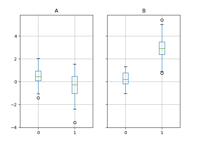
boxplotを呼び出した結果は、キーがグループ化列g（「A」と「B」）の値である辞書です。結果の辞書の値は、boxplotのreturn_typeキーワードで制御できます。詳細については、視覚化ドキュメントを参照してください。

警告

歴史的な理由により、df.groupby("g").boxplot() は df.boxplot(by="g") と等価ではありません。こちらで説明しています。

パイプ関数呼び出し#

DataFrame と Series が提供する機能と同様に、GroupBy オブジェクトを受け取る関数は、pipe メソッドを使用してチェーン接続できます。これにより、よりクリーンで読みやすい構文が可能になります。.pipe の一般的な説明については、こちらを参照してください。

.groupby と .pipe を組み合わせると、GroupBy オブジェクトを再利用する必要がある場合に便利です。

例として、店舗、製品、収益、販売数量の列を持つ DataFrame を考えてみましょう。店舗ごとおよび製品ごとに *価格* （つまり、収益/数量）のグループごとの計算を行いたいとします。これは複数ステップの操作で行うことができますが、パイプを使って表現することで、コードを読みやすくすることができます。まず、データを設定します。

In [265]: n = 1000

In [266]: df = pd.DataFrame(
   .....:     {
   .....:         "Store": np.random.choice(["Store_1", "Store_2"], n),
   .....:         "Product": np.random.choice(["Product_1", "Product_2"], n),
   .....:         "Revenue": (np.random.random(n) * 50 + 10).round(2),
   .....:         "Quantity": np.random.randint(1, 10, size=n),
   .....:     }
   .....: )
   .....: 

In [267]: df.head(2)
Out[267]: 
     Store    Product  Revenue  Quantity
0  Store_2  Product_1    26.12         1
1  Store_2  Product_1    28.86         1

これで、店舗/製品ごとの価格を求めます。

In [268]: (
   .....:     df.groupby(["Store", "Product"])
   .....:     .pipe(lambda grp: grp.Revenue.sum() / grp.Quantity.sum())
   .....:     .unstack()
   .....:     .round(2)
   .....: )
   .....: 
Out[268]: 
Product  Product_1  Product_2
Store                        
Store_1       6.82       7.05
Store_2       6.30       6.64

パイプは、グループ化されたオブジェクトを任意の関数に渡したい場合にも効果的です。たとえば

In [269]: def mean(groupby):
   .....:     return groupby.mean()
   .....: 

In [270]: df.groupby(["Store", "Product"]).pipe(mean)
Out[270]: 
                     Revenue  Quantity
Store   Product                       
Store_1 Product_1  34.622727  5.075758
        Product_2  35.482815  5.029630
Store_2 Product_1  32.972837  5.237589
        Product_2  34.684360  5.224000

ここで、mean は GroupBy オブジェクトを受け取り、それぞれ店舗と製品の組み合わせごとに、収益と数量の列の平均を求めます。mean 関数は、GroupBy オブジェクトを受け取る任意の関数にすることができます。.pipe は、指定した関数に GroupBy オブジェクトをパラメーターとして渡します。

例#

複数列のファクタ化#

DataFrameGroupBy.ngroup() を使用すると、factorize() （リシェイピングAPIで詳しく説明されています）と同様の方法でグループに関する情報を抽出できますが、これは混合型で異なるソースの複数の列に自然に適用されます。これは、グループ行間の関係がその内容よりも重要である場合、または整数エンコーディングのみを受け入れるアルゴリズムへの入力として、処理における中間的なカテゴリのようなステップとして役立ちます。（pandasにおける完全なカテゴリデータのサポートの詳細については、カテゴリの紹介とAPIドキュメントを参照してください。）

In [271]: dfg = pd.DataFrame({"A": [1, 1, 2, 3, 2], "B": list("aaaba")})

In [272]: dfg
Out[272]: 
   A  B
0  1  a
1  1  a
2  2  a
3  3  b
4  2  a

In [273]: dfg.groupby(["A", "B"]).ngroup()
Out[273]: 
0    0
1    0
2    1
3    2
4    1
dtype: int64

In [274]: dfg.groupby(["A", [0, 0, 0, 1, 1]]).ngroup()
Out[274]: 
0    0
1    0
2    1
3    3
4    2
dtype: int64

インデクサによるグループ化によるデータのリサンプリング#

リサンプリングは、既に存在する観測データまたはデータ生成モデルから、新しい仮説的サンプル（リサンプル）を生成します。これらの新しいサンプルは、既存のサンプルと似ています。

日付時刻型ではないインデックスでリサンプリングを機能させるには、次の手順を使用できます。

次の例では、**df.index // 5** は、groupby 操作の選択対象を決定するために使用される整数配列を返します。

注記

以下の例は、サンプルをより少ないサンプルに統合することでダウンサンプリングする方法を示しています。ここでは **df.index // 5** を使用することで、サンプルをビンに集約しています。**std()** 関数を適用することにより、多くのサンプルに含まれる情報を、標準偏差である少数の値のサブセットに集約し、サンプル数を削減しています。

In [275]: df = pd.DataFrame(np.random.randn(10, 2))

In [276]: df
Out[276]: 
          0         1
0 -0.793893  0.321153
1  0.342250  1.618906
2 -0.975807  1.918201
3 -0.810847 -1.405919
4 -1.977759  0.461659
5  0.730057 -1.316938
6 -0.751328  0.528290
7 -0.257759 -1.081009
8  0.505895 -1.701948
9 -1.006349  0.020208

In [277]: df.index // 5
Out[277]: Index([0, 0, 0, 0, 0, 1, 1, 1, 1, 1], dtype='int64')

In [278]: df.groupby(df.index // 5).std()
Out[278]: 
          0         1
0  0.823647  1.312912
1  0.760109  0.942941

名前を伝播させるためのSeriesの返却#

DataFrameの列をグループ化し、一連の指標を計算して、名前付きSeriesを返します。Seriesの名前は、列インデックスの名前として使用されます。これは、スタッキングなどのリシェイピング操作と併用する場合に特に役立ちます。その場合、列インデックスの名前は挿入される列の名前として使用されます。

In [279]: df = pd.DataFrame(
   .....:     {
   .....:         "a": [0, 0, 0, 0, 1, 1, 1, 1, 2, 2, 2, 2],
   .....:         "b": [0, 0, 1, 1, 0, 0, 1, 1, 0, 0, 1, 1],
   .....:         "c": [1, 0, 1, 0, 1, 0, 1, 0, 1, 0, 1, 0],
   .....:         "d": [0, 0, 0, 1, 0, 0, 0, 1, 0, 0, 0, 1],
   .....:     }
   .....: )
   .....: 

In [280]: def compute_metrics(x):
   .....:     result = {"b_sum": x["b"].sum(), "c_mean": x["c"].mean()}
   .....:     return pd.Series(result, name="metrics")
   .....: 

In [281]: result = df.groupby("a").apply(compute_metrics, include_groups=False)

In [282]: result
Out[282]: 
metrics  b_sum  c_mean
a                     
0          2.0     0.5
1          2.0     0.5
2          2.0     0.5

In [283]: result.stack(future_stack=True)
Out[283]: 
a  metrics
0  b_sum      2.0
   c_mean     0.5
1  b_sum      2.0
   c_mean     0.5
2  b_sum      2.0
   c_mean     0.5
dtype: float64

グループ化：分割・適用・結合#

オブジェクトのグループへの分割#

GroupByのソート#

GroupBy dropna#

GroupByオブジェクトの属性#

MultiIndexを使用したGroupBy#

インデックスレベルと列によるDataFrameのグループ化#

GroupByにおけるDataFrame列の選択#

グループの反復処理#

グループの選択#

集約#

組み込み集約メソッド#

aggregate()メソッド#

ユーザー定義関数を使用した集約#

一度に複数の関数を適用する#

名前付き集約#

DataFrame列への異なる関数の適用#

変換#

組み込み変換メソッド#

transform()メソッド#

ウィンドウとリサンプリング操作#

フィルタリング#

組み込みフィルタリング#

filterメソッド#

柔軟なapply#

group_keysによるグループ化された列の配置の制御#

Numbaによる高速化ルーチン#

その他の便利な機能#

数値以外の列の除外#

観測された/観測されていないカテゴリ値の処理#

NAグループの処理#

順序付き因子によるグループ化#

グルーパースペシフィケーションによるグループ化#

各グループの最初の行を取得#

各グループのn番目の行を取得#

グループアイテムの列挙#

グループの列挙#

プロット#

パイプ関数呼び出し#

例#

複数列のファクタ化#

インデクサによるグループ化によるデータのリサンプリング#

名前を伝播させるためのSeriesの返却#

`aggregate()`メソッド#

`transform()`メソッド#

`filter`メソッド#

柔軟な`apply`#

`group_keys`によるグループ化された列の配置の制御#